Universality of Neural Networks on Graphs vs. Sets

November 2022

Petar Veličković, Fabian Fuchs

---

This blog post is a collaboration with Petar Veličković, a colleague at DeepMind, a renowned expert on graph neural networks, and co-author of the Geometric Deep Learning book. This post is a stand-alone article, but in case you have already read my other posts, you can skip the section `Learning on Sets & Universality`. Either way, I hope you enjoy!

Intro

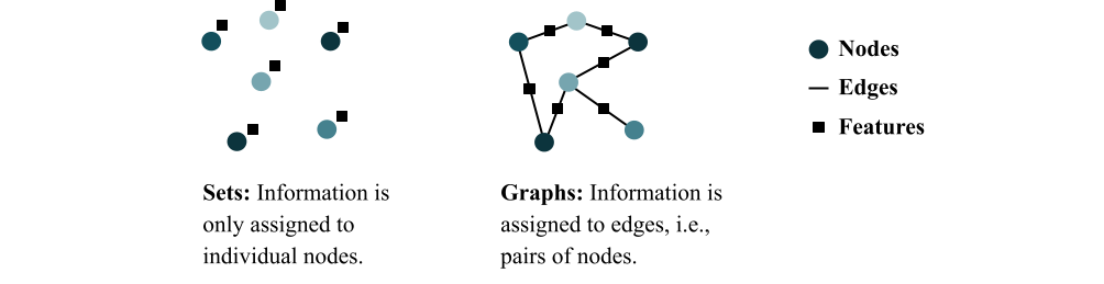
Universal function approximation is one of the central tenets in theoretical deep learning research. It is the question whether a specific neural network architecture is, in theory, able to approximate any function of interest. Specifically in the fields of learning on sets and learning on graphs, universal function approximation is a well-studied property. The two fields are closely linked, because the need for permutation invariance in both cases leads to similar building blocks. The figure below (originally from here) shows that you can think of sets as graphs with just nodes and no edges:

However, these two fields have evolved in parallel, often lacking awareness of developments in the respective other field. This post aims at bringing these two fields closer together, particularly from the perspective of universal function approximation.

Why do we care about universal function approximation?

First of all, why do we need to be able to approximate all functions? After all, having one function that performs well on the train set and generalises to the test set is all we need in most cases. Well, the issue is that we have no idea what such a function looks like, otherwise we would implement it directly and wouldn’t need to train a neural network. Hence, the network not being a universal function approximator may hurt its performance.

Graph Isomorphism Networks (GINs) provide the quintessential example for the merit of universality research: the authors analysed Graph Convolutional Networks (a very popular class of graph neural networks), pointed out that GCNs are not universal, created a varation of the algorithm that is universal (or at least closer to), and achieved better results.

However, this is not always the case. Sometimes, architecture changes motivated by universal function approximation arguments lead to worse results. Even in such unfortunate cases, however, we argue that thinking about universality is no waste of time. Firstly, it brings structure into the literature and into the wide range of models available. We need to group approaches together to see the differences. Universality research can and has served as a helpful tool for that.

Moreover, proving that a certain architecture is or is not universal is an inherently interesting task and teaches us mathematical thinking and argumentation. In a deep learning world, where there is a general sense of randomness and magic in building high-performing neural networks and where it’s hard to interpret what’s going on, one might argue that an additional mathematical analysis is probably good for the balance, even if it turns out to not always directly result in better performance.

Learning on Sets & Universality:

To prove universal function approximation¹, we typically make two assumptions: 1) the MLP components of the neural networks are infinitely large. 2) the functions that we want to be able to learn are continuous on $\mathbb{R}$.

The first part says: any concrete implementation of a ‘universal’ network architecture might not be able to learn the function of interest, but, if you make it bigger, eventually it will—and that is guaranteed ². The second part is a non-intuitive mathematical technicality we will leave uncommented for now and get back to later (because it’s actually a really interesting and important techinicality).

One of the seminal papers discussing both permutation invariant neural networks and universal function approximation was DeepSets in 2017. The idea is simple: apply the same neural network $\phi$ to several inputs, sum up their results, and apply a final neural network $\rho$.

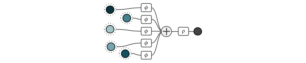
Because the sum operation is permutation invariant, the final output is invariant with respect to the ordering of the inptus. In other words, the sum quite obviously restricts the space of learnable functions to permutation invariant ones. The question is, can a neural network with this architecture, in principle, learn all (continuous) permutation invariant functions. Perhaps surprisingly, the authors show that all functions can indeed be represented with this architecture. The idea is a form of binary bit-encoding in the latent space. Concretely, they argue that there is a bijective mapping from rational to natural numbers. Assuming that each input is a rational number, they first map each rational number $x$ to a natural number $c(x)$, and then each natural number to $\phi(x) = 4^{-c(x)}$. It is now easy to see that $\sum_i \phi(x_i) \neq \sum_i \phi(y_i)$ unless the finite sets $ \{ x_0, x_1, … \} $ and $\{y_0, y_1, …\}$ are the same. Now that we uniquely encoded each input, a universal decoder can map this to any output we want. This concludes the proof that the DeepSets architecture is, in theory, a universal function approximator, despite its simplicity.

However, there is an issue with this proof: it builds on the assumption that the MLP components themselves are universal function approximators, in the limit of infinite width. However, the universal function approximation theorem says that this is the case only for continuous functions, where continuity is defined on the real numbers. That conitnuity is important is sort of intuitive: continuity means that a small change in the input implies a small change in the output. And because the building blocks of neural networks (specifically linear combinations and non-linearities) are continuous, it makes sense that the overall function we want the network to learn should be continuous.

But why continuity on the real numbers? Because continuity on the rational numbers is not a very useful property as shown in Wagstaff et al. 2019. The mapping we described above is clearly highly discontinuous, and anyone could attest that it is completely unrealistic to assume that a neural network could learn such a metric. That doesn’t mean all is lost. Wagstaff et al. show that the DeepSets architecture is still a universal function approximator when requiring continuity, but only if the latent space (the range of $\phi$) has a dimensionality at least as large as the number of inputs, which is an important restriction.

What about graph representation learning?

So, this was universality in the context of machine learning on sets, but what about graphs? Interestingly, the graph representation learning community experienced a near-identical journey, evolving entirely in parallel! Perhaps this observation comes as little surprise: to meaningfully propagate information in a graph neural network (GNN), a local, permutation invariant operation is commonplace.

Specifically, a GNN typically operates by computing representations (“messages”) sent from each node to its neighbours, followed by an aggregation function which, for every node, combines all of its incoming messages in a way that is invariant to permutations. Opinions are still divided on whether every permutation equivariant GNN can be expressed with such pairwise messaging, with a recent position paper from one of the authors (Veličković, 2022) claiming they can. Regardless of which way the debate goes in the future, aggregating messages over 1-hop neighbours gives rise to a highly elegant implementation of GNNs which is likely here to stay. This comes with very solid community backing, with PyG—one of the most popular GNN frameworks—recently making aggregators a “first-class citizen” in their GNN pipelining.

Therefore, to build a GNN, it suffices to build a permutation-invariant, local layer which combines data coming from each node’s neighbours. This feels nearly identical to our previous discussion; what’s changed, really? Well, we need to take care of one seemingly minor detail: it is possible for two or more neighbours to send exactly the same message. The theoretical framework of Deep Sets and/or Wagstaff et al. wouldn’t entirely suffice in this case, as they assumed a set input, whereas now we have a multiset.

Learning on Graphs & Universality:

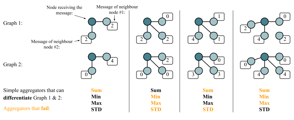
Several influential GNN papers were able to overcome this limitation. The first key development came from the graph isomorphism network (GIN) by Xu, Hu et al. (ICLR’19). GIN is an elegant example of how, over countable features, the maximally-powerful GNN can be built up using similar ideas as in Deep Sets; so long as the local layer we use is injective over multisets. Similarly to before, we must choose our encoder $\phi$ and aggregator $\bigoplus$, such that $\bigoplus\limits_i \phi(x_i) \neq \bigoplus\limits_i \phi(y_i)$ unless the finite multisets $\{ \mkern-4mu \{x_0, x_1, …\} \mkern-4mu \}$ and $\{\mkern-4mu\{y_0, y_1, …\} \mkern-4mu \}$ are the same ($x_i, y_i\in\mathbb{Q}$).

In the multiset case, the framework from Deep Sets induces an additional constraint over $\bigoplus$—it needs to preserve the cardinality information about the repeated elements in a multiset. This immediately implies that some choices of $\bigoplus$, such as $\max$ or averaging, will not yield maximally powerful GNNs.

For example, consider the multisets $\{\mkern-4mu\{1, 1, 2, 2\} \mkern-4mu \}$ and $\{\mkern-4mu\{1, 2\}\mkern-4mu\}$. As we assume the features to be countable, we specify the numbers as one-hot integers; that is, $1 = [1\ \ 0]$ and $2=[0\ \ 1]$. The maximum of these features, taken over the multiset, is $[1\ \ 1]$, and their average is $\left[\frac{1}{2}\ \ \frac{1}{2}\right]$. This is the case for both of these multisets, meaning that both maximising and averaging are incapable of telling them apart.

Summations $\left(\bigoplus=\sum\right)$, however, are an example of a suitable injective operator.

Very similarly to the analysis from Wagstaff et al. in the domain of sets, a similar extension in the domain of graphs came through the work on principal neighbourhood aggregation (PNA) by Corso, Cavalleri et al. (NeurIPS’20). We already discussed why it is a good idea to focus on features coming from $\mathbb{R}$ rather than $\mathbb{Q}$—the universal approximation theorem is only supported over continuous functions. However, it turns out that, when we let $x_i, y_i\in\mathbb{R}$, it is easily possible to construct neighbourhood multisets for which setting $\bigoplus=\sum$ would not preserve injectivity:

In fact, PNA itself is based on a proof that it is impossible to build an injective function over multisets with real-valued features using any single aggregator. In general, for an injective functon over $n$ neighbours, we need at least $n$ aggregation functions (applied in parallel). PNA then builds an empirically powerful aggregator combination, leveraging this insight while trying to preserve numerical stability.

Note that there is an apparent similarity between the results of Wagstaff et al. and the analysis of PNA. Wagstaff et al. shows that, over real-valued sets of $n$ elements, it is necessary to have an encoder representation width at least $n$. Corso, Cavalleri et al. showed that, over real-valued multisets of $n$ elements, it is necessary to aggregate them with at least $n$ aggregators. It appears that potent processing of real-valued collections necessitates representational capacity proportional to the collection’s size, in order to guarantee injectivity. Discovering this correspondence is what brought the two of us together to publish this blog post in the first place, but we do not offer any in-depth analysis of this correspondence here. We do hope it inspires future connections between these two fields, however!

We have established what is necessary to create a maximally-powerful GNN over both countable and uncountable input features. So, how powerful are they, exactly?

The Weisfeiler-Lehman Test

While GNNs are often a powerful tool for processing graph data in the real world, they also won’t solve all tasks specified on a graph accurately! As a simple counterexample, consider any NP-hard problem, such as the Travelling Salesperson Problem. If we had a fixed-depth GNN that perfectly solves such a problem, we would have shown P=NP! Expectedly, not all GNNs will be equally good at solving various problems, and we may be highly interested in characterising their expressive power.

The canonical example for characterising expressive power is deciding graph isomorphism; that is, can our GNN distinguish two non-isomorphic graphs? Specifically, if our GNN is capable of computing graph-level representations \(\mathbf{h}_{\mathcal{G}}\), we are interested whether \(\mathbf{h}_{\mathcal{G_{1}}} \neq\mathbf{h}_{\mathcal{G_{2}}}\) for non-isomorphic graphs \(\mathcal{G}_{1}\) and \(\mathcal{G}_{2}\). If we cannot attach different representations to these two graphs, any kind of task requiring us to classify them differently is hopeless! This motivates assessing the power of GNNs by which graphs they are able to distinguish.

A typical way in which this is formalised is by using the Weisfeiler-Lehman (WL) graph isomorphism test. To formalise this, we will study a popular algorithm for approximately deciding graph isomorphism.

The WL algorithm featurises a graph $\mathcal{G}=(\mathcal{V},\mathcal{E})$ as follows. First, we set the representation of each node $i\in\mathcal{V}$ as $x_i^{(0)} = 1$. Then, it proceeds as follows:

1. Let $\mathcal{X}_i^{(t+1)} = \{\mkern-4mu\{x_j^{(t)} :(i,j)\in\mathcal{E}\}\mkern-4mu\}$ be the multiset of features of all neighbours of $i$.
2. Then, let \(x_i^{(t+1)}=\sum\limits_{y_j\in\mathcal{X}_i^{(t+1)}}\phi(y_j)\), where \(\phi : \mathbb{Q}\rightarrow\mathbb{Q}\) is an injective hash function.

This process continues as long as the histogram of $x_i^{(t)}$ changes—initially, all nodes have the same representation. As steps 1–2 are iterated, certain $x_i^{(t)}$ values may become different. Finally, the WL test checks whether two graphs are (possibly) isomorphic by checking whether their histograms have the same (sorted) shape upon convergence.

While remarkably simple, the WL test can accurately distinguish most graphs of real-world interest. It does have some rather painful failure modes, though; for example, it cannot distinguish a 6-cycle from two triangles!

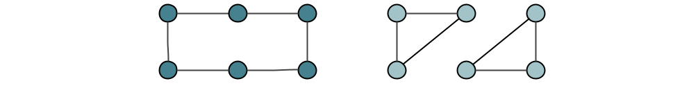
This is because, locally, all nodes look the same in these two graphs, and the histogram never changes.

The key behind the power of the WL test is the injectivity of the hash function $\phi$—it may be interpreted as assigning each node a different colour if it has a different local context. Similarly, we saw that GNNs are maximally powerful when their propagation models are injective. It should come as little surprise then that, in terms of distinguishing graph structures over countable input features, GNNs can never be more powerful than the WL test! And, in fact, this level of power is achieved exactly when the aggregator is injective. This fact was first discovered by Morris et al. (AAAI’19), and reinterpreted from the perspective of multiset aggregation by the GIN paper.

While the WL connection has certainly spurred a vast amount of works on improving GNN expressivity, it is also worth recalling the initial assumption: $x_i^{(0)} = 1$. That is, we assume that the input node features are completely uninformative! Very often, this is not a good idea! It can be proven that even placing random numbers in the nodes can yield to a provable improvement in expressive power (Sato et al., 2021). Further, many recent works (Loukas et al., 2020; Kanatsoulis and Ribeiro, 2022) make it very explicit that, if we allow GNNs access to “appropriate” input features, this leads to a vast improvement in their expressive power.

And, perhaps linking back to our central discussion, focussing only on discrete features may not lead to highly learnable target mapping. From the perspective of the WL test, the model presented in Wagstaff et al., or the PNA model, are no more powerful than 1-WL. However, moving into continuous feature support, PNA is indeed more powerful at distinguishing graphs than models like GIN.