Group CNNs - Equivariance Part 2/2
In our first post, we gave a general introduction to the topic of equivariance. We gave a high-level explanation of how CNNs enforce this property for translations, and outlined the core idea of a method for extending this to more general symmetry transformations. In this post, we’ll see how filling in the details of this outline leads to Group Equivariant Convolutional Networks, as developed by Taco Cohen and Max Welling. We’ll also find out what the little interactive widget above is actually showing us!
As we already have a high-level description of what we’re aiming for from the first post, we’ll dive straight into the mathematics. We’re going to follow the paper pretty closely, concentrating on sections 4, 5 and 6, which contain the bulk of the technical content.
Mathematical Setup
Most of the work in understanding this paper is in getting a proper understanding of the mathematical framework, as covered in section 4. We’ll therefore spend plenty of time on this section, making sure that our grasp of the mathematical setup is rock solid. The first thing we need to nail down is what we mean by symmetry.
Precisely Defining Symmetry
For our purposes, the concept of symmetry is best understood as being defined with respect to a certain property. The property that we’re interested in will vary depending on what task we’re performing. In image classification, for example, the property that we care about is the class of an image. A symmetry with respect to a property is a transformation that leaves the property unchanged. The general setup is as follows:
- We have a set $X$ consisting of all our possible inputs.
- For image classification, $X$ is the space of all images.
- The elements of $X$ have some property of interest. We can view this as a function, $y$, defined on the elements of $X$.
- For image classification, $y$ is the function taking an image to its true class.
- Given a bijective function $g : X \to X$, we say that $g$ is a symmetry with respect to $y$ if, for every $x \in X$:
\begin{equation}
y\big(g(x)\big) = y(x)
\end{equation}
- For image classification, a translation is a symmetry.
The set of all symmetries with respect to $y$ forms a mathematical structure known as a group. This is the “Group” referred to in the title of the paper. For our purposes, a group is always some set of symmetries as defined above1, but the full definition of a group is a bit more general and abstract, and it’s useful to at least have the basics at hand to understand the details of the paper.
Groups, Briefly
A group is a set $G$ together with an operation $*$ which acts on pairs of elements from $G$. For $G$ to qualify as a group, the operation must follow these four rules:
- Closure: $a*b \in G$
- Associativity: $a * (b * c) = (a * b) * c$
- Identity Element: There’s some element $e \in G$ such that $a * e = e * a = a$ for every $a \in G$
- Inverse Elements: Every $a \in G$ has an inverse $a^{-1} \in G$, such that $a * a^{-1} = a^{-1} * a = e$
One useful example of a group is the set of all invertible $n \times n$ matrices, with matrix multiplication as the group operation $*$. If you’re comfortable with linear algebra and you take this as your go-to example of a group, your intuitions will be on pretty safe ground. A familiar property of matrices which turns out to be true for all groups is the following (which is used, for example, in equation 12 of the paper):
\[(a * b)^{-1} = b^{-1} * a^{-1}\]It’s common to omit the $*$ symbol, so instead of the above we can write:
\[(ab)^{-1} = b^{-1} a^{-1}\]Any set of symmetries as discussed above forms a group if we choose to use function composition for the group operation $*$. It’s not too much work to check that the four group properties are satisfied, or you can just trust us!
Some Useful Groups
Cohen and Welling explicitly consider three groups, all of which are symmetry groups for image classification. They’re all defined in terms of functions on $\mathbb{Z}^2$. From here onwards the set $\mathbb{Z}^2$ should be understood as being pixel space, where a pixel is identified with its coordinates $(u, v) \in \mathbb{Z}^2$. We’ll also make use of the so-called homogeneous coordinate system, where $(u, v)$ is written as follows:
\[\left[ {\begin{array}{c} u\\ v\\ 1\\ \end{array} } \right]\]We’re really still looking at a pixel in $\mathbb{Z}^2$ here, but this notation is useful because it allows us to represent the operation of translation as a matrix2.
There’s a subtle but crucial point to notice here. We’ve introduced groups, in our context, as being sets of functions which operate on images. But we’ve just said that we’re going to define some groups of functions on pixels. This distinction is mathematically straightforward to deal with, but we will need to keep it in mind. Let’s define our groups first, and then we’ll see how to bridge the gap between pixel space and image space.
Translation Group: $T$
This is the group of all translations of $\mathbb{Z}^2$. A translation $t \in T$ is a bijective function from $\mathbb{Z}^2$ to $\mathbb{Z}^2$, as required above, and we can write this function as:
\[t(x) = x + (u, v)\]for some integers $u$ and $v$. This naturally associates every $t \in T$ with a point $(u, v) \in \mathbb{Z}^2$, and under this view the group operation (which, recalling from above, is function composition) simply becomes addition. It’s easy to double check this – if we have two translations $t_1, t_2 \in T$, and they correspond to points $(u_1, v_1)$ and $(u_2, v_2)$ as above, then the translation $t_1 \circ t_2$ corresponds to the point $(u_1 + u_2, v_1 + v_2)$.
Since this association between $T$ and $\mathbb{Z}^2$ is very natural, it’s common to simply treat $\mathbb{Z}^2$ as though it is $T$ – this is the convention chosen by Cohen and Welling. If you’re not already comfortable with the mathematics, though, this identification can be confusing, so we’re going to keep these two entities distinct in our notation. For us, $\mathbb{Z}^2$ is pixel space, and $T$ is the group of translations.
Adding Rotations: $p4$
Now we add rotations to the mix. The group $p4$ includes rotations about the origin by $90$ degrees, as well as all the elements of $T$. By the group property of closure, $p4$ must also include the operations that we get by composing translations and rotations. As we know, invertible matrices are a useful example of a group, and Cohen and Welling give an explicit representation of this group as a set of matrices. Any element can be parameterised by three numbers:
- $r$ between $0$ and $3$ – the number of times we rotate by $90$ degrees.
- $u, v \in \mathbb{Z}$ – the translational component of the map.
And we get the following matrix:
\[\left[ {\begin{array}{ccc} \cos(r\pi/2) & -\sin(r\pi/2) & u\\ \sin(r\pi/2) & \cos(r\pi/2) & v\\ 0 & 0 & 1\\ \end{array} } \right]\]This matrix rotates and translates a 2D point represented in the homogeneous coordinate system described above.
Adding Reflections: $p4m$
Here we just add a reflection operation to $p4$ (and, again, we’ll need to include all compositions to maintain closure). We now get a parameterisation by four numbers – $r, u,$ and $v$ as above, and:
- $m$ either 0 or 1 – the number of times we reflect
And again we have an explicit representation of every element of this group as a matrix:
\[\left[ {\begin{array}{ccc} (-1)^m\cos(r\pi/2) & (-1)^{m+1}\sin(r\pi/2) & u\\ \sin(r\pi/2) & \cos(r\pi/2) & v\\ 0 & 0 & 1\\ \end{array} } \right]\]We now have three groups, each of which captures different symmetries of image classification:
- $T$ captures translational symmetry.
- $p4$ captures both translational and rotational symmetry.
- $p4m$ captures all three of translational, rotational and reflective symmetry.
Recall from above that these groups all act on pixels, not images. As promised, we’re now going to see how to talk about these groups operating instead on image space.
Acting on Images – What’s $L_g$?
A quick note to keep our terminology straight: we’ll stick with Cohen and Welling in viewing an image (or a CNN feature map) as a function on pixel space, i.e. an assignment of a colour (or an activation) to each pixel. Now, on to business.
Let’s consider a translation $t$ from the translation group $T$ defined above, and suppose we have some image $f$. To talk about a translated version of $f$, it seems most natural to write $t(f)$. Since we haven’t defined $t$ to act on images, however, this expression doesn’t make sense. $t$ is a function on pixels, and $f$ is not a pixel. So we need to define a new function, $L_t$, which represents the same translation, but is a function on images instead of pixels.
This $L_t$ is defined in a counterintuitive way:
\begin{align} L_t(f) &= f \circ t^{-1} \newline \big(L_t(f)\big)(x) &= f\big(t^{-1}(x)\big) \end{align}
Where does this $t^{-1}$ come from? Why not just $t$? To see where this comes from, we’ll again need to think about two different perspectives on the same operation. The first perspective is an image being translated over a fixed field of pixels – this is the translated version of $f$ that we care about, $L_t(f)$. The second perspective is a field of pixels being translated under a fixed image – exactly the same operation, from a different viewpoint. But now think about, for instance, translating an image to the right. If we switch to the “moving pixels, fixed image” perspective, the pixels are moving to the left relative to the image. In general, when we switch to the “moving pixels, fixed image” perspective, the pixels will move in the opposite direction to the motion of the image. So as shown in the video below, an image shifting over by $t$ is equivalent to the pixels shifting over by $t^{-1}$.
This definition doesn’t just work for translation. It holds for all symmetry groups. Transforming the image by a symmetry operation $g$ is the same as transforming the pixels by $g^{-1}$, and $L_g$ is just Cohen and Welling’s notation for “transforming the image by $g$”. Cohen and Welling also omit the parentheses when applying $L_g$ to $f$, and simply write $L_g f$ instead of $L_g(f)$, but these are just two ways of writing exactly the same thing. We’ll follow their notation from now on to avoid an explosion of parentheses!
Translation Equivariance of CNNs
Now we’re equipped to understand the proofs from the paper. We’ll start with section 5, showing that the translation equivariance of a standard CNN can be proved nicely within this framework.
First let’s write down the definition of convolution:
\begin{align} (f\star \psi)(x) &= \sum_{y\in \mathbb{Z}^2} \sum_{k=1}^{K}f_k(y)\psi_k(y-x) \end{align}
Technically speaking, this defines a correlation, not a convolution. The convention in the deep learning world, though, is to call this a convolution, and we’ll be sticking with this convention.
Here, $\psi$ and $f$ both have $K$ channels. For the rest of this post, we’ll take $K=1$ for brevity, as do Cohen and Welling. Keeping the sum over $k$ is a trivial alteration to the proofs.
Now let’s briefly remind ourselves what the goal is here. We have an image $f$, and we’re going to convolve it with a filter $\psi$ to get a map of activations. Then we want to know that, for any translation $t$, the following two operations are the same:
- Translate $f$ by $t$, and convolve the result with $\psi$.
- Convolve $f$ with $\psi$, and translate the result by $t$.
So the equation we want is:
\[(L_tf) \star \psi = L_t (f \star \psi)\]This defines exactly what we mean when we say “convolution is equivariant with respect to $T$”.
Proof
We’ll prove this slightly differently from the proof given in the paper, by noting that we can rewrite the convolution with the substitution $y \mapsto x+y$:
\begin{align} (f \star \psi)(x) &= \sum_{y\in \mathbb{Z}^2} f(y)\psi(y - x) \newline &= \sum_{y\in \mathbb{Z}^2} f(x + y)\psi(y) \end{align}
Now we just write out the definition of both sides of the equation we want to show, and we immediately get the result. First, the definition of $(L_t f) \star \psi$:
\begin{align} \big((L_tf) \star \psi\big)(x) &= \big((f \circ t^{-1}) \star \psi\big)(x) \newline &= \sum_{y\in \mathbb{Z}^2} f\big(t^{-1}(x + y)\big)\psi(y) \newline &= \sum_{y\in \mathbb{Z}^2} f(x + y - t)\psi(y) \end{align}
And the definition of $L_t (f \star \psi)$:
\begin{align} \big(L_t(f \star \psi)\big)(x) &= (f \star \psi)(x - t) \newline &= \sum_{y\in \mathbb{Z}^2} f\big((x - t) + y\big)\psi(y) \newline &= \sum_{y\in \mathbb{Z}^2} f(x + y - t)\psi(y) \end{align}
These two expressions are equal, so we’re done.
It’s worth thinking about what exactly we’ve done here. Most of the above was just writing out the definitions of $L_t$ and $\star$. The only real content of our proof was in rewriting the definition of convolution, substituting $y \mapsto x + y$. Let’s look at this definition again:
\[\sum_{y\in \mathbb{Z}^2} f(y)\psi(y - x) = \sum_{y\in \mathbb{Z}^2} f(x + y)\psi(y)\]Think back to the first post, where we talked about the equivalence between the single-image-many-filters perspective and the single-filter-many-images perspective. The equation above is exactly this equivalence, just written more formally. Every term in the sum on the left hand side has the same image, and its own transformed version of the filter. The opposite is true on the right hand side – every term has the same filter, and its own transformed version of the image.
Hopefully, relating this back to the high-level explanation given in the last post makes it clear that this equivalence is true. It’s also worth thinking a little more formally about why it holds. The substitution $y \mapsto x+y$ that we made to show this equivalence works for two reasons:
- This substitution is a bijection from $\mathbb{Z}^2$ to $\mathbb{Z}^2$.
- The sum is over the entire space $\mathbb{Z}^2$.
These two properties together ensure that every term that appears in the sum on the left-hand side also appears in the sum on the right-hand side, and vice versa.
Interestingly, this reasoning also matches with the practical limitations of translation equivariance in CNNs. Convolutional layers are not perfectly translation equivariant because we always lose information at the boundaries. In other words, in practice, we do not sum over all of $\mathbb{Z}^2$, but only over a subset. This violates point 2 above, so the substitution doesn’t quite hold.
For reference, the original proof from the paper is as follows:
\begin{align} \big((L_t f)\star\psi\big)(x) &= \sum_y f(y-t) \psi(y-x) \newline &= \sum_y f(y) \psi(y+t-x) \newline &= \sum_y f(y) \psi\big(y-(x-t)\big) \newline &= \big(L_t (f\star\psi)\big)(x) \end{align}
The corresponding crucial step here is at the second equals sign, with the substitution $y \mapsto y + t$. This substitution is justified for exactly the same reasons and is the main content of this version of the proof.
Unfinished Business
We made a promise in part one, and it’s time for us to pay up. Towards the end of the post, we developed some intuition about how to achieve equivariance. We broke this down into two parts:
- When computing the convolution $f \star \psi$, we consider many transformed versions of the image $f$. If we later need to compute the convolution for a transformed copy of $f$, we can just go and look up the relevant outputs, because we’ve already computed them.
- We can perform the lookup by transforming the output in the same way as we transformed $f$.
We justified point 1, and we said that we’d have to wait for this second post to justify point 2. We’ve justified everything above line-by-line, but you might feel that we still don’t have much insight into why point 2 holds – we’ll spend the next few paragraphs digging into this, and we’re going to carry on making use of our mathematical definitions from above.
First, take another look at our rewritten definition of convolution:
\[(f \star \psi)(x) = \sum_{y\in \mathbb{Z}^2} f(y + x)\psi(y)\]What job is $x$ doing here? We’re viewing it as an element of $\mathbb{Z}^2$, but all it’s actually doing in this equation is being added to $y$ – that is, it’s performing a translation. As we’ve noted before, we can view any $x \in \mathbb{Z}^2$ as naturally corresponding to an element $t$ of our translation group $T$. So let’s do it – same equation, new perspective:
\[(f \star \psi)(t) = \sum_{y\in \mathbb{Z}^2} f\big(t(y)\big)\psi(y)\]Here, we’re explicitly thinking about the convolution in terms of translations, which matches up more naturally with our “many transformed versions of $f$” description. This also generalises nicely if we want to transform $f$ with other groups like $p4$ and $p4m$ – we’ll come back to that later. We’ve pulled our definition of convolution a bit closer to the intuitive picture, and we can now take this process a bit further. This is a tricky bit aimed at solidifying a deeper understanding of what’s going on, and it’s not essential. So if you’re feeling maths fatigue, skip ahead to Group Equivariance In General.
Still with us? Let’s look a little more closely at the last equation, and how it relates to our points 1 and 2 above.
- In point 1, we talked about “transformations of $f$”. We now know how to formalise this with $L_g$. Looking at the right hand side, we can see that our transformation of $f$ is just $f \circ t$. That is, it’s $L_{t^{-1}}f$.
- In point 2, we said that we need to transform our output. The output we’re talking about here is the whole function $f \star \psi$. Again, we know how to formalise this transformation with $L_g$. Seeing which $L_g$ to use is a bit more tricky, but if we write the left hand side as $(f \star \psi)(t(\mathbf{0}))$3 we can see that the situation is the same as on the right – we’re looking at $(f \star \psi) \circ t$, which is $L_{t^{-1}}(f \star \psi)$.
So we can just tweak the mathematical language of our equation so that it matches up more closely with the prose in points 1 and 2. For notational sanity we’ll let $\tau = t^{-1}$.
\[L_{\tau}(f \star \psi)(\mathbf{0}) = \sum_{y\in \mathbb{Z}^2} L_{\tau}f(y)\psi(y)\]On the left we’re transforming the output as in point 2, and on the right we have the transformed version of the image from point 1. This new way of writing the definition of convolution matches very closely with our high-level description from last time. Referring back to any of our earlier definitions of convolution, it’s obvious that the right hand side is just the convolution $L_{\tau}f \star \psi$ evaluated at $\mathbf{0}$. So we’ve already got an instance of equivariance, just by reworking the definition:
\[L_{\tau}(f \star \psi)(\mathbf{0}) = (L_{\tau}f \star \psi)(\mathbf{0})\]This line of reasoning can be extended to show equivariance in general, but we’ll stop here to prevent this post from collapsing under its own weight4.
Group Equivariance in General
Finally, we’re at the heart of the paper. We’ve shown that the mathematical framework accounts for translation equivariance in CNNs, and now we’ll show that, by a very similar mechanism, we can get any kind of group equivariance we like! We’re going to start with ordinary convolution as defined above, and work our way towards defining Cohen and Welling’s $G$-convolution. A reminder about terminology here – in their paper, Cohen and Welling do pay attention to the distinction between convolution and correlation mentioned above. To maintain consistency with the deep learning convention, we’re going to carry on saying convolution, but in the paper, this is (correctly!) referred to as correlation.
With that out of the way, let’s take a look at our group-flavoured definition of convolution from above:
\[(f \star \psi)(t) = \sum_{y\in \mathbb{Z}^2} f\big(t(y)\big)\psi(y)\]Is there anything special about $T$? Can’t we do this for any symmetry group on $\mathbb{Z}^2$? Indeed we can! If we now let $g \in G$, we can define the first layer $G$-convolution:
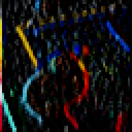
\[(f \star \psi)(g) = \sum_{y \in \mathbb{Z}^2} f\big(g(y)\big)\psi(y)\]There’s a potential point of confusion here – what sort of function is $f \star \psi$? In normal convolution, the inputs to $f \star \psi$ were pixels, but now the inputs are group elements – that is, $f \star \psi$ is a function on $G$. That’s fine in the abstract, but how do we get a concrete handle on how to think about it? For a general group $G$, thinking concretely might be very hard, but all of our groups are thankfully pretty friendly. $T$ is basically just $\mathbb{Z}^2$, so we can think of these functions as looking like images as normal. We’ll come back to talking about $p4$ and $p4m$ later on, but the right hand side of the visualisation at the top of this post is just a $p4$ feature map – that is, a function on $p4$.
So $f \star \psi$ having group-valued inputs isn’t too scary5, but it does pose a problem for us. We only know how to convolve functions with $\mathbb{Z}^2$-valued inputs. We don’t yet know how to take our output function and convolve it with something else. Right now we’re stuck with a single-layered network – so much for deep learning!
How To Go Deeper
If we want to build a deep network of $G$-convolutions, we need to be able to convolve $f \star \psi$ with another filter, and convolve the result with something else, and just keep on convolving. Thankfully, another straightforward modification to our definition of $G$-convolution will allow us to do this. Suppose $f$ and $\psi$ are now defined on $G$, instead of $\mathbb{Z}^2$. We can $G$-convolve them as follows:
\[(f\star \psi)(g) = \sum_{h\in G} f(gh)\psi(h)\]Where, since $g$ and $h$ are both elements of $G$, $gh$ just means the group composition $g * h$.
This is the definition of $G$-convolution, and we can show that it’s equivariant with respect to $G$ in the same way as we did for the CNN above. First, let’s remind ourselves of what we want to show. Letting $u \in G$ because we’re running out of letters, we want:
\[(L_u f) \star \psi = L_u (f \star \psi)\]Expanding the definition of $(L_u f) \star \psi$:
\begin{align} \big((L_u f) \star \psi\big)(g) &= \big((f \circ u^{-1}) \star \psi\big)(g) \newline &= \sum_{h\in G} f(u^{-1}gh)\psi(h) \end{align}
And the definition of $L_u (f \star \psi)$:
\begin{align} \big(L_u(f \star \psi)\big)(g) &= (f \star \psi)(u^{-1}g) \newline &= \sum_{h\in G} f(u^{-1}gh)\psi(h) \end{align}
These two expressions are equal, so we’re done.
Again, all we’ve done is expand definitions, and the real content was in the definition of $G$-convolution. We’ve rewritten the definition given in the paper, in essentially the same way we did for the CNN case. The original definition from the paper is:
\[(f\star \psi)(g) = \sum_{h\in G} f(h)\psi(g^{-1}h)\]Our rewriting of this corresponds to the substitution $h \mapsto gh$, and once again this corresponds to the crucial line of the proof in the original paper, where the substitution is $h \mapsto uh$.
Leftovers
There are still a couple of things left to address here.
Firstly, when $f$ and $\psi$ are just an ordinary image and a filter, defined on $\mathbb{Z}^2$ (i.e. in the first layer of our network), we’ll be using the first layer $G$-convolution that we defined above:
\[(f \star \psi)(g) = \sum_{y \in \mathbb{Z}^2} f\big(g(y)\big)\psi(y)\]Showing that this is also an equivariant operation can be done in exactly the same way as the proofs above.
Secondly, we noted above that what we’ve been calling convolution should really be referred to as correlation. So what’s a true convolution? Is it also $G$-equivariant? The true convolution is defined as follows:
\[(f * \psi)(g) = \sum_{h\in G} f(h)\psi(h^{-1}g)\]Again it’s helpful to rewrite this with the substitution $h \mapsto gh$, to get this equivalent definition:6
\[(f * \psi)(g) = \sum_{h\in G} f(gh)\psi(h^{-1})\]This definition is easily plugged into all the proofs above to show that, yes, this operation is also $G$-equivariant.
That’s A Wrap
Good news – we’re done with the maths! We haven’t covered 100% of what’s in the paper – for example we’ve missed out the other elements you need to build a full $G$-CNN. Convolutional networks don’t only consist of convolutions, after all, and Cohen and Welling also consider e.g. pooling layers. If you’ve got this far, though, you should be pretty well equipped to go straight to the paper and absorb the rest of what’s there.
We said above that we’d talk a bit about how to visualise the feature maps produced by $G$-convolution, so we’ll finish the post with a brief discussion of that, and an encore appearance of the visualisation at the top of the page.
Visualisation of the $G$-Convolution
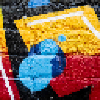
Now that we’ve defined $G$-convolution, let’s see what rotation equivariance looks like in practice for the p4 symmetry group. This interactive visualisation lets you translate and rotate the input image on the left, and shows the corresponding first-layer feature map on the right7. Intermediate-layer feature maps also look similar to the right hand side, as do intermediate-layer convolutional filters (compare with figure 1 in the paper).
As with the animation of convolution in our first post, nothing is really in motion here. In reality, we only have four discrete rotations available to us – the continuous animation just makes things more intuitive8.
Photo credit: Kyle Van Alstyne
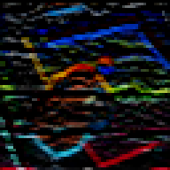
Note that normally, the feature map would have dimensions $h\times w$. Here, we have $h\times w \times 4$ because of the four $90^\circ$ rotations – we view this as having 4 separate $h\times w$ patches. The above visualisation isn’t the only way we could choose to arrange these 4 patches, but it gives us a very natural way to visualise how rotations affect the feature map.
How can we visualise the computation of these first layer activations? The same filter is effectively applied 4 times in different orientations. We can see this in the visualisation – the filter is a dark-to-light edge detector, and each patch shows edges in different orientations. The top patch shows left-to-right edges. The left patch shows bottom-to-top edges, a difference of $90^\circ$, and so on. What happens if we rotate the input image by $90^\circ$? Then the left-to-right filter applied to the original image should produce the same outcome as the bottom-to-top filter applied to a one-time-rotated-image – just rotated by $90^\circ$.
With $p4m$, the picture is not too different – we just have an additional 4 patches, one each for the reflected version of the $p4$ patches.
Conclusion
That’s it! In this two-post series, we gave a general introduction to the concept of equivariance, linked it to neural networks and CNNs in particular, and explained Group Equivariant Convolutional Networks. While this approach provides some generality and is not restricted to translations, rotations and mirroring, it cannot be easily extended to, e.g., continuous rotations. However, this is a very active area of research with a large body of follow-up work addressing the limitations of this approach (e.g., Harmonic Networks, Steerable CNNs, 3D Steerable CNNs, Learning to Convolve). For instance, just a few days ago, LieConv (code here) was introduced. It’s a CNN simultaneously applicable to images, molecular data, dynamical systems, and other arbitrary continuous data. LieConv can be made equivariant to a wide range of continuous matrix groups by defining continuous parametric kernels over elements of the Lie algebra, the vector space of infinitesimal transformations from the group. We’re sure that there’s plenty of further interesting work to come!
Credit: Ed is funded by the EPSRC Centre for Doctoral Training in Autonomous Intelligent Machines and Systems. I am funded by the Bosch Center for AI where I am currently undertaking a research sabbatical. A big thank you also to Daniel Worrall for a number of conversations on this topic, and Adam Golinski and Mike Osborne for proofreading and feedback.
-
Note for group-theory-savvy readers: yes, this set of symmetries is most naturally understood in terms of an action of some underlying group. In this post we only care about faithful actions, which preserve all of the group structure, so we’re going to gloss over this. ↩
-
We can’t do this in ordinary $\mathbb{Z}^2$ because translation is nonlinear – it doesn’t fix the origin. ↩
-
We’ll write $\mathbf{0}$ for the identity translation, or if you prefer the $\mathbb{Z}^2$ description, this is the point $(0, 0)$. ↩
-
Or in more traditional language, we leave this as an exercise for the reader 🙂 ↩
-
Although getting comfortable with the visualisation might take a while – playing around with the interactive widget should help! ↩
-
If the equivalence isn’t clear, recall from our discussion of groups that $(gh)^{-1} = h^{-1}g^{-1}$, so under our substitution we get $\psi(h^{-1}g) \mapsto \psi(h^{-1}g^{-1}g) = \psi(h^{-1})$. ↩
-
i.e. the output of the first convolution. ↩
-
And, crucially, makes the visualisation more fun to play with! ↩