Permutation Invariance, DeepSets and Universal Function Approximation
This is a blog post by Ed Wagstaff, Martin Engelcke and me about if and when the DeepSets architecture limits universal function approximation. The post is very closely related to our 2019 ICML paper On the Limitations of Representing Functions on Sets, but should be significantly easier to process. We wrote the post in collaboration with Ferenc Huszár and hosted it on his website. The links to our images on Ferenc’s website are currently broken. In the meantime, I copied the blog post here:
Ferenc: One of my favourite recent innovations in neural network architectures is Deep Sets. This relatively simple architecture can implement arbitrary set functions: functions over collections of items where the order of the items does not matter.
This is a guest post by Fabian Fuchs, Ed Wagstaff and Martin Engelcke, authors of a recent paper on the representational power of such architectures and why the deep sets architecture can represent arbitrary set functions in theory. It’s a great paper. Imagine what these guys could achieve if their lab was in Cambridge rather than Oxford!
Here are the links to the original Deep Sets paper, and the more recent paper by the authors of this post:
- Zaheer, Kottur, Ravanbakhsh, Poczos, Salakhutdinov and Smola (NeurIPS 2017) Deep Sets
- Wagstaff, Fuchs, Engelcke, Posner and Osborne (ICML 2019) On the Limitations of Representing Functions on Sets
Over to Fabian, Ed and Martin for the rest of the post. Enjoy.
Sets and Permutation Invariance in ML
Most successful deep learning approaches make use of the structure in their inputs: CNNs work well for images, RNNs and temporal convolutions for sequences, etc. The success of convolutional networks boils down to exploiting a key invariance property: translation invariance. This allows CNNs to
- drastically reduce the number of parameters needed to model high-dimensional data
- decouple the number of parameters from the number of input dimensions, and
- ultimately, to become more data efficient and generalize better.
But images are far from the only data we want to build neural networks for. Often our inputs are sets: sequences of items, where the ordering of items caries no information for the task in hand. In such a situation, the invariance property we can exploit is permutation invariance.
To give a short, intuitive explanation for permutation invariance, this is what a permutation invariant function with three inputs would look like: \(f(a,b,c)=f(a,c,b)=f(b,a,c)=\ldots\)
Some practical examples where we want to treat data or different pieces of higher order information as sets (i.e. where we want permutation invariance) are:
- working with sets of objects in a scene (think AIR or SQAIR)
- multi-agent reinforcement learning
- perhaps surprisingly, point clouds We will talk more about applications later in this post.
Note from Ferenc: I would like to jump in here - because it’s my blog so I get to do that - to say that I think the killer application for this is actually meta-learning and few-shot learning. By meta-learning, don’t think of anything fancy, I consider amortized variational inference, like a VAE, as a form of meta-learning. Consider a conditionally i.i.d model where you have a global parameter θ, and a bunch of observations $x_i$ drawn conditionally i.i.d from a distribution $p(X\vert \theta)$. Given a set of observations $x_1,\ldots, x_N$ we’d like to approximate the posterior $p(\theta\vert x_1,\dots,x_N)$ by some parametric $q(\theta\vert x_1,\ldots,x_N;\psi)$, and we want this to work for any number of observations $N$. Clearly, the real posterior $p$ has a permutation invariance with respect to xn, so it would make sense to make the recognition model, $q$, a permutation-invariant architecture. To me, this is the killer application of deep sets, especially in an on-line learning setting, where one wants to update our posterior estimate over some parameters with each new data point we observe.
The Deep Sets Architecture (Sum-Decomposition)
Having established that there is a need for permutation-invariant neural networks, let’s see how to enforce permutation invariance in practice. One approach is to make use of some operation $P$ which is already known to be permutation-invariant. We map each of our inputs separately to some latent representation and apply our $P$ to the set of latents to obtain a latent representation of the set as a whole. $P$ destroys the ordering information, leaving the overall model permutation invariant.
In particular, Deep Sets does this by setting $P$ to be summation in the latent space. Other operations are used as well, e.g. elementwise max. We call the case where the sum is used sum-decomposition via the latent space. The high-level description of the full architecture is now reasonably straightforward - transform your inputs into some latent space, destroy the ordering information in the latent space by applying the sum, and then transform from the latent space to the final output. This is illustrated in the following figure:
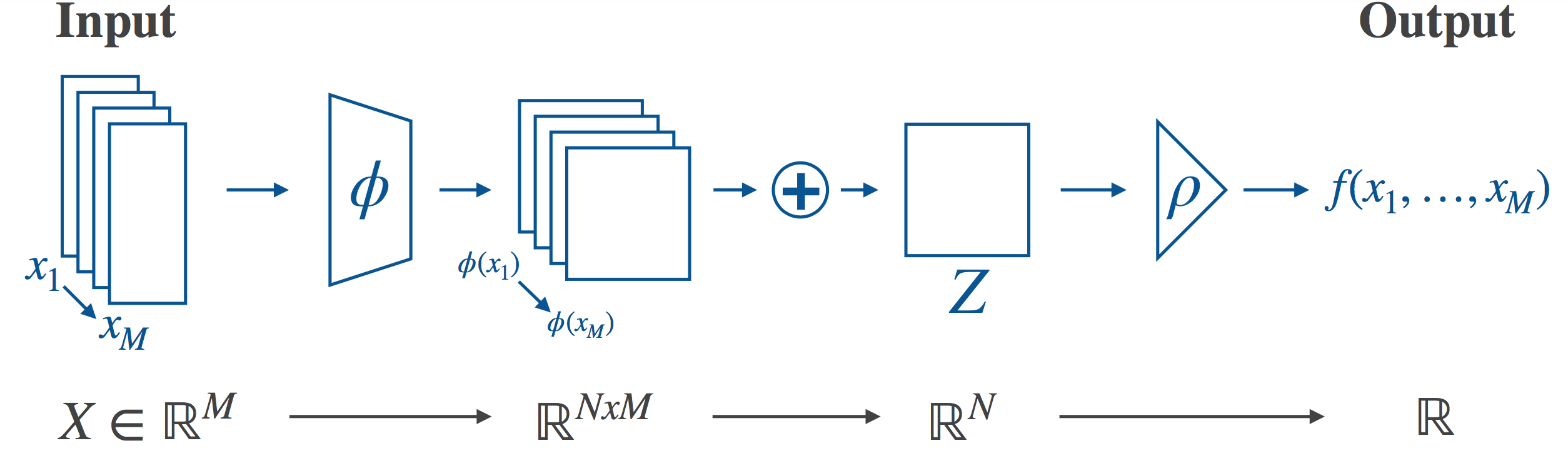
If we want to actually implement this architecture, we’ll need to choose our latent space (in the guts of the model this will mean something like choosing the size of the output layer of a neural network). As it turns out, the choice of latent space will place a limit on how expressive the model is. In general, neural networks are universal function approximators (in the limit), and we’d like to preserve this property. Zaheer et al. provide a theoretical analysis of the ability of this architecture to represent arbitrary functions - that is, can the architecture, in theory, achieve exact equality with any target function, allowing us to use e.g. neural networks to approximate the necessary mappings? In our paper, we build on and extend this analysis, and discuss what implications it has for the choice of latent space.
Can we get away with a small latent space?
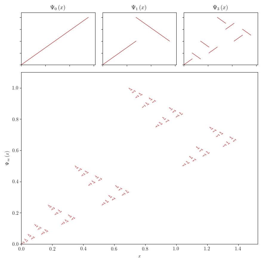
Zaheer et al. show that, if we’re only interested in sets drawn from a countable domain (e.g. ℤ or ℚ), a 1-dimensional latent space is enough to represent any function. Their proof works by defining an injective mapping from sets to real numbers. Once you have an injective mapping, you can recover all the information about the original set, and can, therefore, represent any function. This sounds like good news – we can do anything we like with a 1-D latent space! Unfortunately, there’s a catch – the mapping that we rely on is not continuous. The implication of this is that to recover the original set, even approximately, we need to know the exact real number that we mapped to – knowing to within some tolerance doesn’t help us. This is impossible on real hardware.
Above we considered a countable domain, but it’s important to consider instead the uncountable domain ℝ, the real numbers. This is because continuity is a much stronger property on ℝ than on ℚ, and we need this stronger notion of continuity. The figure below illustrates this, showing a function which is continuous on ℚ but not continuous on ℝ (and certainly not continuous in an intuitive sense). The figure is explained in detail in our paper. Using ℝ is particularly important if we want to work with neural networks. Neural networks are universal approximators for continuous functions on compact subsets of $ℝ^M$. Continuity on ℚ won’t do.
Zaheer et al. go on to provide a proof using continuous functions on ℝ, but it places a limit on the set size for a fixed finite-dimensional latent space. In particular, it shows that with a latent space of $M+1$ dimensions, we can represent any function which takes as input sets of size $M$. If you want to feed the model larger sets, there’s no guarantee that it can represent your target function.
As for the countable case, the proof of this statement uses an injective mapping. But the functions we’re interested in modeling aren’t going to be injective – we’re distilling a large set down into a smaller representation. So maybe we don’t need injectivity – maybe there’s some clever lower-dimensional mapping to be found, and we can still get away with a smaller latent space?
No.
As it turns out, you often do need injectivity into the latent space. This is true even for simple functions, e.g. max, which is clearly far from injective. This means that if we want to use continuous mappings, the dimension of the latent space must be at least the maximum set size. We were also able to show that this dimension suffices for universal function representation. That is, we’ve improved on the result from Zaheer (latent dimension $N\geq M+1$ is sufficient) to obtain both a weaker sufficient condition, and a necessary condition (latent dimension $N\geq M$ is sufficient and necessary). Finally, we’ve shown that it’s possible to be flexible about the input set size. While Zaheer’s proof applies to sets of size exactly $M$, we showed that $N=M$ also works if the set size is allowed to vary $\leq M$.
Applications & Connections
Why do we care about all of this? Sum-decomposition is in fact used in many different contexts - some more obvious than others - and the above findings directly apply in some of these.
Attention Mechanisms
Self-attention via {keys, queries, and values} as in the Attention Is All You Need paper by Vaswani et al. 2017 is closely linked to Deep Sets. Self-attention is itself permutation-invariant unless you use positional encoding as often done in language applications. In a way, self-attention “generalises” the summation operation as it performs a weighted summation of different attention vectors. You can show that when setting all keys and queries to 1.0, you effectively end up with the Deep Sets architecture.
Therefore, self-attention inherits all the sufficiency statements (‘with $N=M$ you can represent everything’), but not the necessity part: it is not clear that $N=M$ is needed in the self-attention architecture, just because it was proved that it is needed in the Deep Sets architecture.
Working with Point Clouds
Point clouds are unordered, variable length lists (aka sets) of $xyz$ coordinates. We can also view them as (sparse) 3D occupancy tensors, but there is no ‘natural’ 1D ordering because we have three equal spatial dimensions. We could e.g. build a kd-tree but again this imposes a somewhat ‘unnatural’ ordering.
As a specific example, PointNet by Qi et al. 2017 is an expressive set-based model with some more bells and whistles. It handles interactions between points by (1) computing a permutation-invariant global descriptor, (2) concatenating it with point-wise features, (3) repeating the first two steps several times. They also use transformer modules for translation and rotation invariance — So. Much. Invariance!
Stochastic Processes & Exchangeability A stochastic process corresponds to a set of random variables. Here we want to model the joint distributions of the values those random variables take. These distributions need to satisfy the condition of exchangeability, i.e. they need to be invariant to the order of the random variables.
Neural Processes and Conditional Neural Processes (both by Garnelo et al. 2018) achieve this by computing a global latent variable via summation. One well-known instance of this is Generative Query Networks by Eslami et al. 2018 which aggregate information from different views via summation to obtain a latent scene representation.
Summary
👋 Hi, this is Ferenc again. Thanks to Fabian, Ed and Martin for the great post.
Update: As commenters pointed out, these papers are, of course, not the only ones dealing with permutation invariance and set functions. Here are a couple more things you might want to look at (and there are quite likely many more that I don’t mention here - feel free to add more in the comments section below)
- Vinyals et al, 2015 on handling permutation invariance in the seq2seq framework.
- Lee et al, 2018 proposed an attention-based architecture to implement set functions.
- Bloem-Reddy and Teh, 2019 for a more theoretical take on invariances in neural networks.
As I said before, I think that the coolest application of this type of architecture is in meta-learning situations. When someone mentions meta-learning many people associate to complicated “learning to learn to learn via gradient descent via gradient descent via gradient descent” kind of things. But in reality, simpler variants of meta-learning are a lot closer to being practically useful.
Here is an example of a recommender system developed by Vartak et al, 2017 for Twitter, using this idea. Here, a user’s preferences are summarized by the set of tweets they recently engaged with on the platform. This set is processed by a DeepSets architecture (the sequence in which they engaged with tweets is assumed to carry little information in this application). The output of this set function is then fed into another neural network that scores new tweets the user might find interesting.
Such architectures can prove useful in online learning or streaming data settings, where new datapoints arrive over time, in a sequence. For every new datapoint, one can apply the $\phi$ mapping, and then simply maintain a moving averages of these $\phi$ values. For binary classification, one can have a moving average of $\phi(x)$ for all negative examples, and another moving average for all positive examples. These moving averages then provide a useful, permutation-invariant summary statistics of all the data received so far.
In summary, I’m a big fan of this architecture. I think that the work of Wagstaff et al (2019) provides further valuable intuition on their ability to represent arbitrary set functions.