Gumbel Softmax

This post introduces the Gumbel Softmax estimator for stochastic neural networks. It was simultaneously discovered by Maddison et al. and Jang et al., with both papers published at ICLR 2017. I took figures, equations and notation from the latter of the two.

Vanilla Gumbel Softmax Estimator

The Gumbel Softmax trick can be looked at from different angles. I will approach it from an attention angle, which has a broad range of applications in deep learning. For example, imagine a neural network that processes an image and decomposes it into multiple objects. Now we want it to continue with just one (e.g. the most ‘relevant’) object and want our neural network to do something with it. In other words, we want the neural network to attend to this specific object.

This form of attention is discrete or hard, whereas usually, in neural networks, we perform soft attention because it is easier to backpropagate through. Often, hard attention is more intuitively suited for the problem, but we find a way of approximating it with soft attention instead (making the process differentiable). E.g. in MOHART, each object tracker attends to an image region. Intuitively, we would crop the image and just process the image crop. However, it is not straight-forward to differentiate the parameters for the crop in order to have the network learn where to attend to. So instead, we soften the boarders with Gaussians.

Similarly, in Attention Is All You Need (an NLP paper), the self-attention module does not discretely attend to a specific word but takes a weighted sum of the word embeddings.

In some situations, however, we want an approach which comes closer to hard attention than a weighted sum. We specifically look at setups where we want the network to attend to an element of a set. This is where Gumbel Softmax comes into play, which combines two tricks. Let’s assume the attention scores $\pi_i$ are outputs of a softmax and can therefore be seen as class probabilities $\left(\sum \pi_i = 1,\, \pi_i \geq 0 \forall i \right)$. The Gumbel-Max trick offers an efficient way of sampling from this categorical distribution by adding a random variable to the log of the probabilities and taking the argmax:

\[z=\text { one_hot }\left(\underset{i}{\arg \max }\left[g_{i}+\log \pi_{i}\right]\right)\]

where $g_i$ are i.i.d. samples drawn from a Gumbel distribution. The key here is that the samples $z$ are identical to samples from the categorical distribution. Why not sample from the categorical distribution directly? This is an instance of the reparameterization trick known from VAEs. By sampling $g$ from a fixed distribtution and reparameterizing this distribtution using $\pi$, we avoid having to backpropagate through the stochastic node (the sampling of $g$) and instead only backpropagate into the determinstic reparameterization, updating the probabilities $\pi_i$.

The second step is to replace the argmax with a softmax to make this operation differentiable as well:

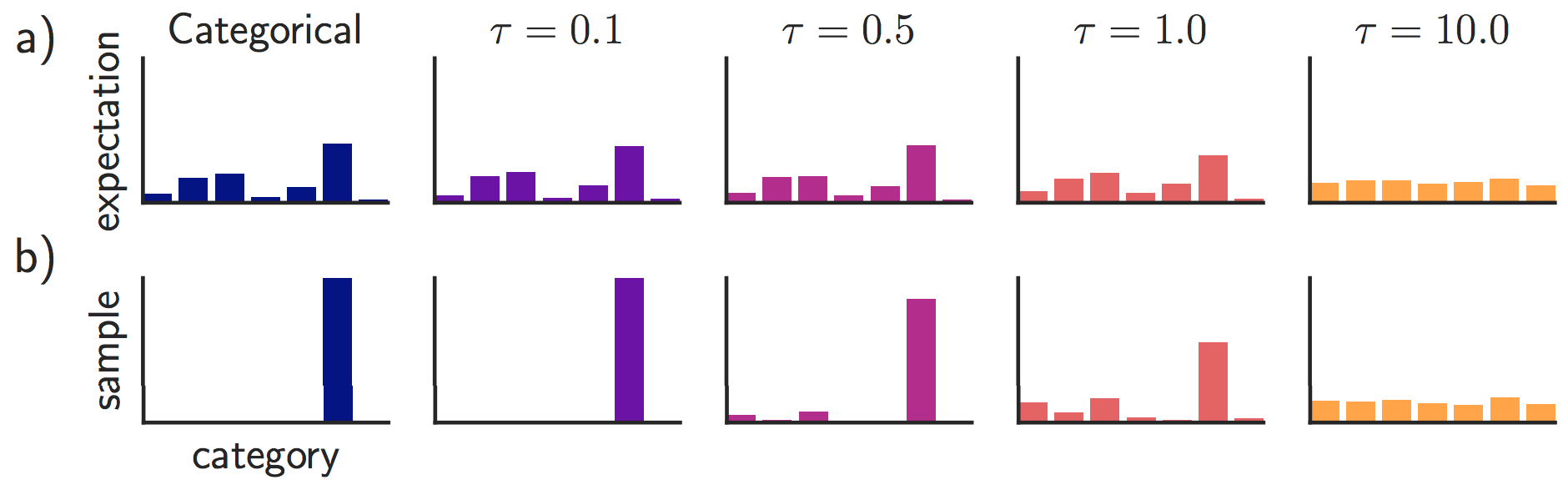
\[y_{i}=\frac{\exp \left(\left(\log \left(\pi_{i}\right)+g_{i}\right) / \tau\right)}{\sum_{j=1}^{k} \exp \left(\left(\log \left(\pi_{j}\right)+g_{j}\right) / \tau\right)}\]

Importantly, the softmax here has a temperature parameter $\tau$. Setting $\tau$ to 0 makes the distribution identical to the categorical one and the samples are perfectly discrete as shown in the figure below. For $\tau \to \inf$, both the expectation and the individual samples become uniform:

Drawbacks of Gumbel Softmax

(1) For $\tau > 0$, the distribution is not identical to the true categorical distribution (as can be seen in the figure above). This means that this procedure is a biased estimator of the true gradients.

(2) For small $\tau$, the gradients have high variance, which is a typical issue of stochastic neural networks. Hence, there is a trade-off between variance and bias.

(3) For $\tau > 0$, the samples are not discrete, hence we do not actually perform hard attention. Rather it is just closer, i.e. peakier, than softmax (compare expectation for $\tau=0.0$ and samples for $\tau \leq 1.0$ in figure above).

A Variation: Straight-Through Gumbel Softmax

This version of the Gumbel Softmax estimator introduces a trick which allows us to set $\tau$ to 0 (i.e. performing hard attention), but still estimate gradients.

When $\tau=0$, the softmax becomes a step function and hence does not have any gradients. The straight-through estimator is a biased estimator which creates gradients through a proxy function in the backward pass for step functions.

This trick can also be applied to the Gumbel Softmax estimator: in the equations above, $z$ (using argmax) was the true categorical distribution wheras $y$ (using softmax) is the continuous relaxation and hence an approximation. In the straight-through version, the argmax version is used in the forward pass but the softmax version is used in the backward pass, hence approximating the true gradients $\nabla_\theta z$ with $\nabla z \approx \nabla y$.

An Alternative: REINFORCE

An alternative way of estimating the gradients is the score function estimator (SF), also known as REINFORCE, which is an unbiased estimator. In a stochastic neural network parameterized by $\theta$, we seek to optimise the expectation value with respect to the distribution over samples $z$: $\nabla E_z[f(z)]$

We can pull the gradient operator into the integral and use the identity $\nabla p(z) = p(z) \nabla\log p(z)$ to rewrite the above expression as: $E_z[f(z)\nabla \log p(z)]$

REINFORCE itself has been around for a while (Williams, 1992), but there have been advances in recent years on how to combat the high variance in gradients which is introduced with this method. This can be achieved by adding a function b(z) within the integral and subtracting the expectation value of this function. This keeps the value of the overall expectation the same while (if b(z) is chosen well) potentially reducing the variance.

Open Questions about Gumbel Softmax

The following are my own thoughts about the Gumbel Softmax Estimator as someone who has never actually worked with stochastic neural networks and just read about them. I’d be happy about any feedback!

1) For $\tau > 0$, the Gumbel Softmax is a continuous relaxation of the discrete sampling and therefore can be seen of soft attention. This makes the process differentiable with respect to the parameters $\pi_i$. A benefit of this formulation is that we can easily switch from soft to hard attention by changing the temperature parameter. This, however, brings us to the first open question:

Could we simply introduce the same temperature parameter in the softmax used in the self-attention module and have the same benefit of being able to switch between soft and hard attention during test time?

The obvious difference to softmax with temperature is the stochastic component of adding $g_i$ to the logits. This introduces stochasticity into the process and is a fundamental difference to most other forms of attention used in neural networks. The potential benefit for me is that this avoids local minima during training time:

Imagine the network picks a specific object to attend over and which turns out to be a reasonable choice. The gradients might tell the network that it gets better results when taking a ‘purer’ form of the representation of this object, i.e. making that distribution peakier. However, this may ignore the possibility that there is another object which is even better to attend to. The stochasticity of the Gumbel Softmax, therefore, helps exploration.

2) If this avoidance of local minima is the main benefit of the stochasticity, this brings me to my second open question:

Why do we add the Gumbel noise during test time?

My current take on this: We only want to add the noise during test time if we want our network to be stochastic due to the nature of its application. In Reinforcement Learning, for example, stochasticity in the actions (even during test time) might allow for more effective exploration of the state space. In a recommendation system set-up without access to the history of previous recommendations, stochasticity avoids showing the same recommendation each time. However, in many applications stochasticity might not give any benefits during test time and would just decrease performance. In those cases, I do not see any reason why not to set $g_i = 0$ during test time.