Review: Deep Learning on Sets

Fabian Fuchs, Ed Wagstaff, Martin Engelcke

---

In this blog, we analyse and categorise the different approaches in set based learning. We conducted this literature review as part of our recent paper Universal Approximation of Functions on Sets with Michael Osborne and Ingmar Posner.

Credit: Last year, I sent out a tweet to the hive mind. We wanted to understand why so many neural network architectures for sets resemble either Deep Sets or self-attention. The answers were very insightful and allowed us to write this blog. A sincere thank you to Thomas Kipf, William Woof, Zhengyang Wang, Christian Szegedy, Daniel Worrall, Bruno Ribeiro, Marc Brockschmidt, Paul-Edouard Sarlin, Chirag Pabbaraju and many others!

In Machine Learning, we encounter sets in the form of collections of inputs or feature vectors. Crucially, these collections have no intrinsic ordering, which distinguishes them from image or audio data. Examples with this property are plentiful: point clouds obtained from a LIDAR sensor, a group of atoms which together form a molecule, or collections of objects in an image. In all of these scenarios, neural networks are regularly employed. Set-based problems are a bit different from other deep learning tasks such as image classification. When classifying a molecule¹ based on the constituent atoms and their locations, it shouldn’t matter in which order we list the atoms. This symmetry gives us the chance to build a useful inductive bias into the network. The model could learn to not care about orderings, but that would be a waste of training data and computation time if we also have the option to make it permutation invariant by design.²

In this blog post, we examine deep learning architectures that are suited to work with set data. The core question here is: how do we design a deep learning algorithm that is permutation invariant while maintaining maximum expressivity? We tried to find a mece (mutually exclusive, collectively exhaustive) division of the methods out there into four different paradigms, which also make up the four sections of this blog post:

• Permuting & Averaging
• Sorting
• Approximating Invariance
• Learning on Graphs

Whether perfectly mece or not, we hope that this provides the reader with some structure and overview over this fast growing field. Enjoy!

Permuting & Averaging

There are a wide array of models available within Deep Learning. Can we modify such existing models to be permutation-invariant, rather than coming up with something entirely new? There are multiple ways to do this.

The first is the permuting & averaging paradigm. It works as follows: consider all possible permutations of our input elements, pass each permutation through a permutation-sensitive model separately, and then take the average of all the results. If two inputs $\mathbf{x}$ and $\mathbf{y}$ are permutations of one another, this process will clearly give the same output for both inputs. We can write this mathematically as:

\[\widehat{f}(\mathbf{x}) = \frac{1}{|S_N|} \sum_{\pi \in S_N} \phi \bigl( \pi \left( \mathbf{x} \right) \bigr)\]

where $\mathbf{x}$ has $N$ elements, and $S_N$ is the set of all permutations of $N$ elements. We thereby construct a permutation-invariant $\widehat{f}$ from a permutation-sensitive $\phi$.

This idea is known as Janossy pooling and was introduced by Murphy et al. While it is a very straightforward way of getting exact permutation invariance, it’s also extremely computationally expensive. The expense comes from the sum over $S_N$. The number of elements of $S_N$ is $N!$, so as the size of the sets under consideration increases, this sum quickly becomes intractable.

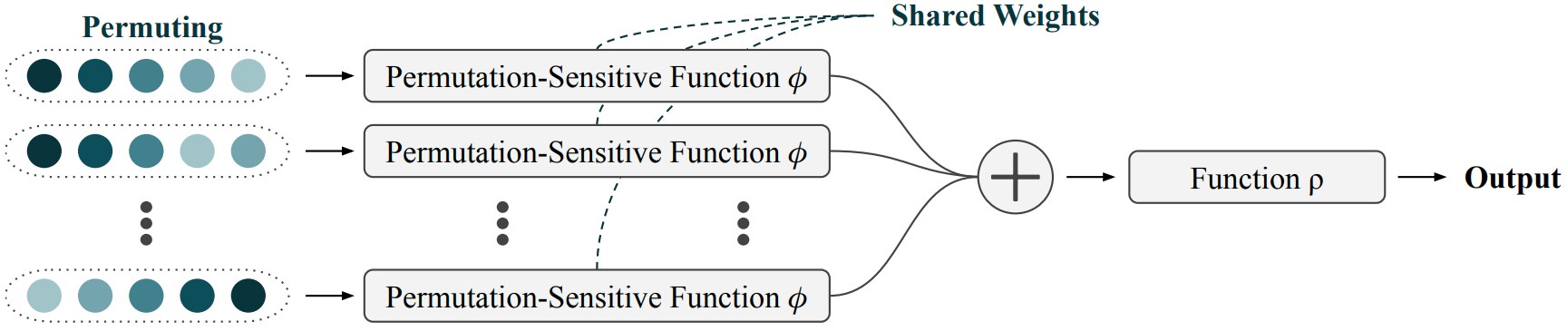
In the diagram above, $\widehat{f}$ comprises everything up to and including the sum. The function $\rho$ coming after the sum is optional and does not need to follow any constraints to guarantee invariance because its input, $\widehat{f}(\mathbf{x})$, is already invariant. Put another way, the ordering information is already lost by this point in the diagram. Adding the optional block after the sum can greatly enhance the expressivity of the model (at least in theory).

Limiting the Number of Elements in Permutations

To save some computation, we can give up on permuting all $N$ elements. In the above, we look at all possible $N$-tuples from an $N$ element set, but what if we instead consider all $k$-tuples,³ for some $k < N$? This was suggested by Murphy et al., as a way of building computationally less expensive models that are still permutation-invariant. Letting $\mathbf{x}_{{k}}$ stand for a $k$-tuple from $\mathbf{x}$, we have:

\[\widehat{f}(\mathbf{x}) = \sum_{\mathbf{x}_{\{k\}}} f(\mathbf{x}_{\{k\}})\]

As with Janossy pooling, we’ll actually want to divide through by the number of terms in the sum – we’ll count the number of terms shortly. First it’s worth considering a quick example to clarify exactly what this expression is doing. Suppose our input set with $N=4$ is ${w, x, y, z}$, and we set $k=2$. Then our sum will be over all 2-tuples from our set, namely:

\((w, x),~(x, w),(w, y),~(y, w),~(w, z),~(z, w), \\ (x, y),~(y, x),~(x, z),~(z, x),~(y, z),~(z, y)\)

The sum over all of these tuples is clearly invariant to permutations of the elements of the input set – each tuple will still appear exactly once in the sum, no matter how we shuffle the individual elements around.

Now how many terms are there in our sum? The number of $k$-tuples from a set of $N$ elements is:

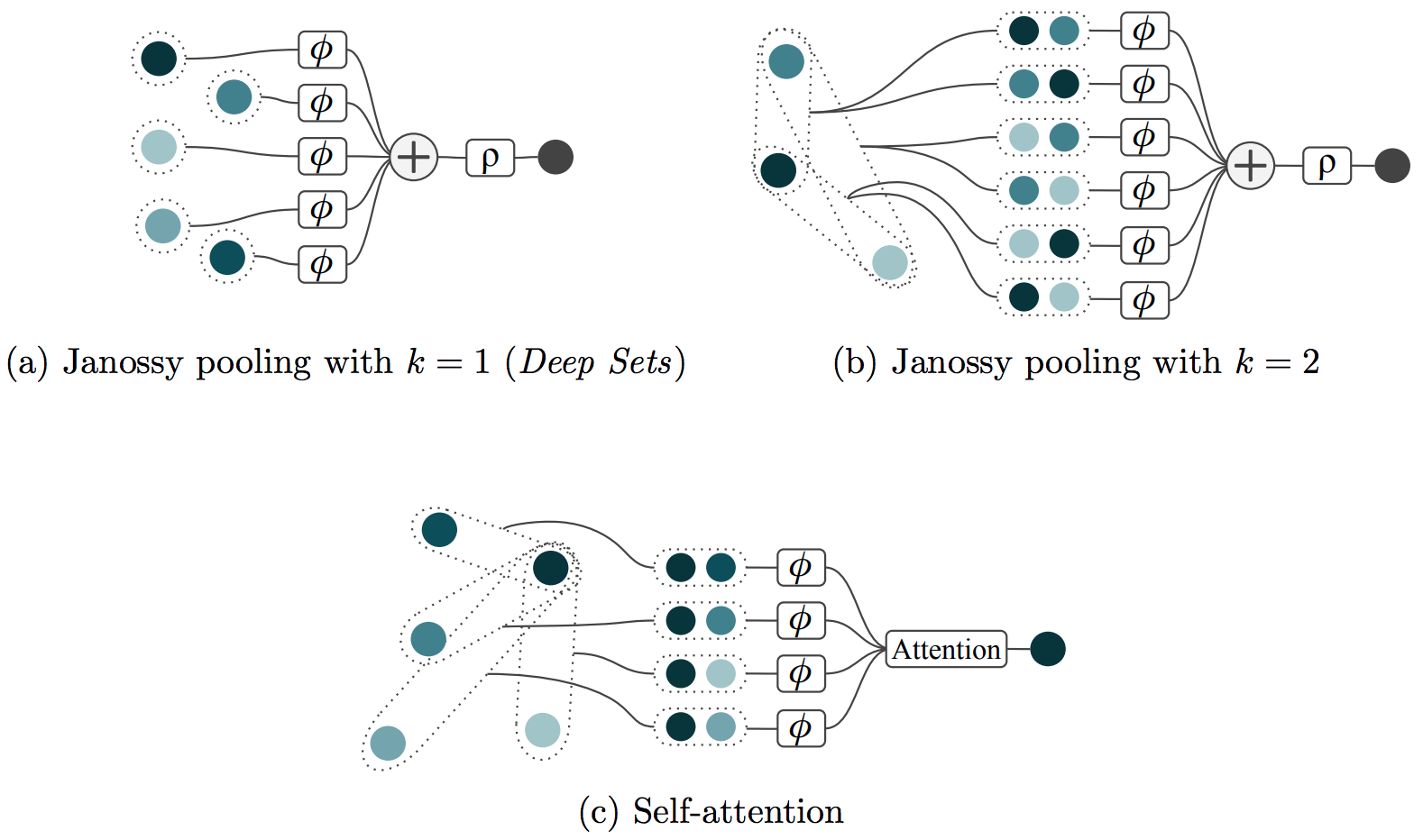
\[P(N,k) = N!/(N-k)!\]

For sufficiently small $k$, this is so much better than $N!$ that it gives us a tractable method. Setting $k=N$ gives us the most expressive—and most expensive—model. Setting $k=1$ gives us a model whose cost is linear in the size of the input set. Increasing $k$ lets us take into account higher-order interactions between elements in the set – we’ll come back to this idea of interactions later in this post.

Deep Sets

Setting $k=1$, and including the optional function $\rho$, we obtain a well known special case, Deep Sets. The authors propose a neural network architecture in which each input is first transformed by a neural network $\phi$ individually. The results are then aggregated via a sum and further processed by a second neural network $\rho$. Perhaps thanks to its linear scaling in computation time, this approach became quite popular and is the basis of two famous point cloud classification approaches: PointNet and PointNet++. In On the Limitations of Representing Functions on Sets, we showed that this architecture guarantees universal function approximation for all permutation invariant functions if the dimension of network $\phi$’s output is at least as large as the number of inputs.⁴ This means, that in the limit of infinitely sized networks $\phi$ and $\rho$, $k=1$ is technically sufficient. However, this doesn’t mean that other architectures with $k>1$ don’t yield better results in practice. In the next paragraph, we explore a concrete reason why that might be.

Expressivity and Interactions

You may have come across the terms relational reasoning and interactions. These are often used without definitions or in-depth explanations, so let’s give it a go:

When we talk about interactions between elements in a set, we’re really trying to capture the fact that our output may depend not only on the individual contribution of each element, but it may be crucial to also take into account the fact that certain elements appear together in the same set. Relational reasoning simply describes the act of modelling and using these interactions.

To illustrate this with a simple example, consider the task of assessing how well a set of ingredients go together for cooking a meal. If we set $k=1$, the function $\phi$ can take into account relevant individual attributes, but will be unable to spot any clashes between ingredients (like garlic and vanilla). Increasing $k$ allows $\phi$ to see multiple elements at once, and therefore perform relational reasoning about pairs of ingredients, enabling a more expressive model of what tastes good. If we view $\phi$ as an encoder'' and $\rho$ as adecoder’’, $\phi$ is capable of encoding information about interactions, which $\rho$ can then make use of during decoding.

When we increase $k$ here, we give ourselves the ability to take these interactions into account explicitly. If we use Deep Sets, even with $k=1$, we can take these interactions into account implicitly. This is because the “back half” of the model (i.e. neural network $B$ from the previous section), which gets the encoded set as its input⁵, sees the whole set at once. So, in principle, it’s capable of taking into accout interactions between any number of elements, and could learn these implicitly. However, the version of the set that it sees is a learned encoding, so it’s harder to design the model so that it makes use of these interactions.

Self-Attention

Perhaps exactly because of this enhanced relational reasoning, a lot of current neural network architectures on graphs and sets actually resemble binary Janossy pooling (i.e. $k=2$). Most famously, self-attention algorithms compare two elements of the set at a time, typically by performing a scalar product. The results of the scalar products are used as attention weights for aggregating information from different points via a weighted, permutation invariant sum. While this mechanism is very similar to Janossy pooling with $k=2$, there is a bit more going on. For example, often a softmax is used to ensure that the attention weights sum up to 1.

To concretise the relationship between the permutation invariant binary Janossy pooling and self-attention, let’s first define a natural extension of k-ary Janossy pooling from invariance to equivariance. In regular binary Janossy pooling, a function $\phi$ acts on all two-tuples followed by a sum-pooling. Purely for visualisation, we write those two-tuples in a matrix:

\[\begin{pmatrix} \phi(x_1, x_1) & \phi(x_2, x_1) & \cdots & \phi(x_N, x_1) \\ \phi(x_1, x_2) & \phi(x_2, x_2) & \cdots & \phi(x_N, x_2) \\ \vdots & & \ddots & \vdots \\ \phi(x_1, x_N) & \phi(x_2, x_N) & \cdots & \phi(x_N, x_N) \end{pmatrix}\]

Pooling over the entire matrix gives an invariant output. Pooling over each row individually gives a permutation equivariant output. In general we define k-ary equivariant Janossy pooling as follows: output $i$ is optained by aggregating over all ($\phi$-transformed) k-tuples which start with element $x_i$. A second network $\rho$ may then further transform each output individually.

Specifically for binary equivariant Janossy pooling, this reads:

\[f_i(\mathbf{x}) = \rho \left( \sum_j \phi(x_i, x_j) \right)\]

In practice, $\phi(x_i, x_j)$ is usually split up in attention weights $w(x_i, x_j)$ and values $v(x_j)$ and a softmax acts on the weights. However, the binary Janossy pooling character very much remains with every element in the above matrix being covered exactly once.

Sorting

When we represent a set as an ordered structure, we generally assume that the order can be arbitrary. That is, we can have two representations $\mathbf{x}$ and $\mathbf{y}$ of the same set, where the elements are ordered differently, and we regard both of these as valid representations of the set. We could instead say that each set has only one valid representation, corresponding to some canonical ordering of the elements. If we ensure that only this valid representation is ever seen by our model, by first sorting the elements, then we’ll get permutation invariance.

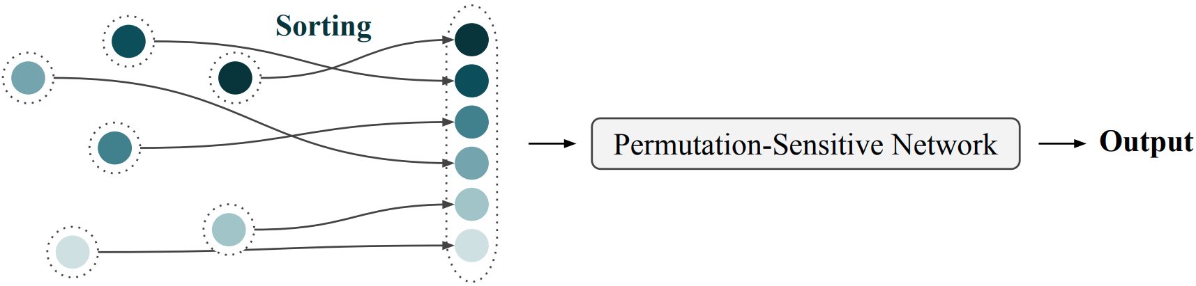
This is much cheaper than the permuting and averaging method. The only extra cost here is the cost of sorting the elements into their canonical representation, which is $O(n~\text{log}n)$. There are a couple of issues still worth discussing with this method.

First there’s a question of how to pick the canonical ordering. This choice can be made manually, but the choice of ordering may in fact affect the performance of the model. We can instead learn this ordering – or more straightforwardly, we can learn a function which gives a score to each element, and then sort the elements by their scores. This brings us to the second issue – how do we train this model? More specifically, how do we get gradients for this scoring function?

The ranking of elements according to their sorting score is a piece-wise constant function⁶, meaning that the gradients are zero almost everywhere (and undefined at the remaining places). This wouldn’t be a problem if we had labels for the perfect ranking during training time – then we could just predict the ranking and get losses & gradients by comparing it to the ground truth. But we don’t have labels for the perfect ranking. A good ranking is whatever allows the decoder (the permutation sensitive network) to perform well. This makes getting proper gradients a lot more difficult. However, it’s not the first time we’ve encountered the problem of needing to backpropagate through piecewise constant functions in deep learning. The straight-through estimator, for example, is a viable tool. Recently, a cheap differentiable sorting operation has been proposed by Blondel et. al, with a computational cost of $O(n~\text{log}\,n)$. To the best of our knowledge, this hasn’t been applied to standard set-based deep learning tasks, but this area could ccertainly provide interesting applications of this method.

The authors of Non-Local Graph Neural Networks choose yet another approach: after ranking the inputs according to a learned score function, they apply a 1D convolution to the ranked values. However, in order to get gradients for the score function, they multiply each value with its score before feeding it into the convolutional layer. The interesting bit is that, while the gradients do backpropagate into the score function, they don’t come from the sorting. The gradients come from the scores being used as features later on. This is a similar prinicple as in FSPool, where Zhang et al. sort features according to their values and then directly use those features as input for the next layer. However, the auto-encoder variant of FSPool comes with a continuous relaxation approach to estimating sorting gradients and is therefore closer in spirit to the straight-through estimator approach described in the previous paragraph.

Approximate Permutation Invariance

While setting $k<N$ is an appealing way to avoid the cost of considering all permutations as discussed, it might not be the best solution in all situations. Murphy et al. therefore also propose an alternative approximate/stochastic solution: let’s stick with $k=N$, but instead of averaging over all possible permutations $P(N,k)$, we can randomly sample an arbitrary number of permutations $p<P(N,k)$ and only average over those to achieve approximate permutation invariance. This approximation becomes exact as $p \rightarrow P(N,k)$.

Murphy et al. show that this even works quite well when setting $p=1$. We could also use, for example, $p=1$ during training and $p>1$ at test time when we care more about the fidelity of our predictions, akin to ensemble methods. Maybe this would even be a way to obtain uncertainty estimates for our predictions?

Pabbaraju & Jain approximate permutation invariance with a very different approach. Inspired by Generative Adversarial Networks, they propose to use an adversary that tries to find the permutations of the input data which yield maximum loss values. This encourages the model to become close to permutation-invariant to minimise the impact of the adversary.

From Sets to Graphs

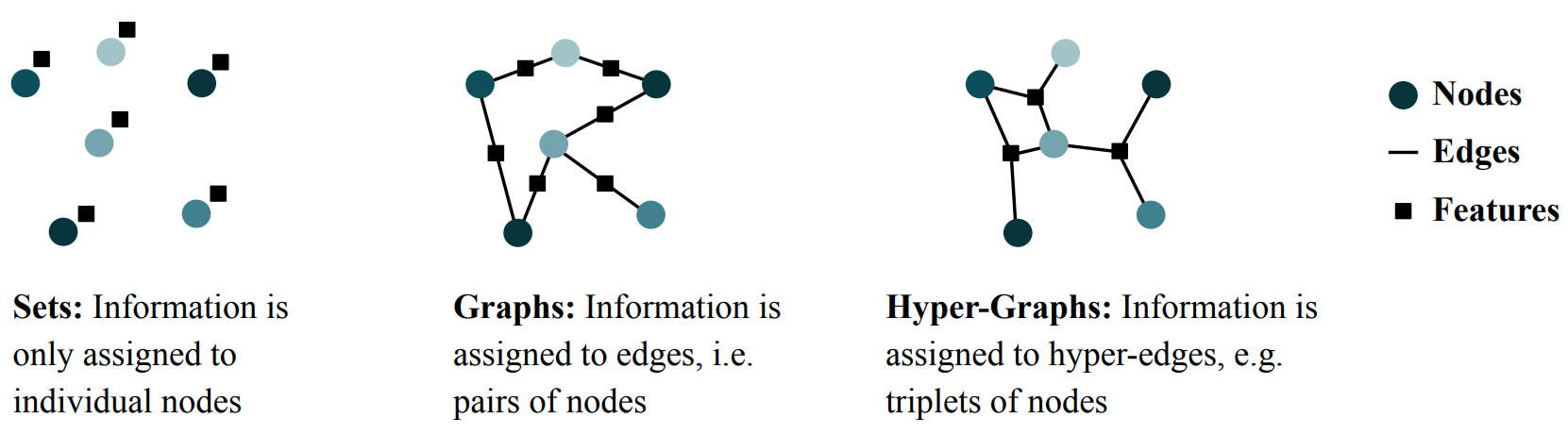
So far, we have been talking about mechanisms on sets, but there is also an interesting connection to graphs. Graphs typically consist of nodes and edges, where each edge connects two nodes. This can be extended to hyper-graphs which include information attached to triplets of nodes (e.g. HyperGCN, LambdaNet). From this perspective, it becomes clear that a set can be seen as a graph without edges. Interestingly, there is no canonical way to apply Deep Sets to graphs, because it is not clear how to process the edge information. With self-attention algorithms, on the other hand, it is very simple to include edge information (see, e.g., Section 3.3 in SE(3)-Transformers).

Notably, Maron et al. study the set of independent linear, permutation-invariant or equivariant functions (i.e. matrices) transforming vectorised versions of the adjacency tensors. In fact, there is an orthogonal basis of such linear, permutation-equivariant functions. The number of basis vectors is connected to the \textit{Bell number} and is, remarkably, independent of the number of nodes in the (hyper-)graph. As an example, the edge information of a bi-directional graph can be written as an $M \times M$ adjacency matrix or, after vectorising this matrix, as a vector of length $M^2$. This vector can now be linearly transformed by multiplying it with a matrix of size $M^2 \times M^2$. Maron et al. show that there is an orthogonal basis of 15 different $M^2 \times M^2$ matrices which transform the (vectorised) adjacency matrix in an equivariant manner. The number 15 is the fourth Bell number, and is independent of the size $M$ of the graph.

Conclusion

Before we started with the research for this blog post, we realised that almost all of the algorithms for sets that we were aware of were variations of either Deep Sets or Self-Attention. Both seemed like pretty arbitrary architecture choices. The Janossy Pooling framework gives a satisfying explanation: these two algorithms are just the two most scalable cases ($k=1$ & $k=2$) of the permuting and averaging paradigm. If you found this post interesting, have a look at the full paper, Universal Approximation of Functions on Sets. Also, drop us a message any time and let us know what you thought of the blog post, the paper, or both. :)

---