AlphaFold 2 and Iterative SE(3)-Transformers

Ed Wagstaff & Fabian Fuchs

Find the accompanying paper here (selected for oral presentation at the International Conference on Geometric Science of Information, Paris, 2021).

In a previous blog post, Justas & Fabian explained how iterative 3D equivariance was used in AlphaFold 2. To summarise, equivariance leverages the symmetry of the problem, i.e. the fact that the global orientation of the protein is meaningless and should not interfere with the reasoning about its structure. Concretely, the structure module of AlphaFold 2 uses a network that is mathematically guaranteed to produce equivalent outputs for rotated versions of the input. We also stated that SE(3)-Transformers can be used to build such a 3D equivariant structure module. However, there is one part we previously glanced over: the structure module of AlphaFold 2 is applied iteratively. In each step, it takes an estimate of atom coordinates as an input to a 3D equivariant network and predicts updates. It then uses the updated positions as an input for the next iteration. Such a use case was not intended in the original SE(3)-Transformer paper and it comes with a few challenges which we aim to address in this blog post and the accompanying tech report. We make the code available here.

Background: Fibers

We will assume that the reader of the rest of this post is familiar with the concept of equivariance. If not, we recommend either the blog post about AlphaFold 2 and equivariance or the first part of our earlier blog post on equivariance as an introduction. In this section we’ll dig a little deeper into the SE(3)-Transformer itself, and introduce the concept of fibers¹. We’ll explain fibers on a reasonably high level, but feel free to dive deeper into the maths by reading the paper, especially appendices A and B.

In the SE(3)-Transformer,² everything transforms in an equivariant way, including all the features of the graph. This has some implications for how we define those features. For instance, there are two possible ways in which a three-dimensional feature can be equivariant – when applying a rotation to the graph, we can either rotate the feature along with the graph (this is how we would treat a feature encoding velocity, for example) or we can leave it unchanged (this is how we would treat RGB colour information). When we define a feature, we therefore need to choose not only its dimension, but also which transformation rule it obeys. We give these “features with transformation rules” a new name to distinguish them from ordinary features, and call them fibers.

The transformation rules for three-dimensional fibers are straightforward, but typically we have high-dimensional features in the hidden layers of a neural network. We might reasonably want, say, a 64-dimensional fiber in the intermediate layers of an SE(3)-Transformer. What does it mean for such a fiber to transform under a 3D rotation? It turns out that there is a surprisingly neat way to define the transformation rules for any fiber. Ultimately, a high-dimensional fiber can be viewed as a concatenation of multiple lower-dimensional fibers. Let’s look at a concrete example to see what this looks like.

Consider a toy problem where we have 2 particles with initial locations $\vec{x_1},\vec{x_2}$ and velocities $\vec{v}_1,\vec{v}_2$. Our task is to predict new positions $\vec{x}^\prime_1, \vec{x}^\prime_2$. Such a task is typically equivariant: rotating input positions and velocities with a $3\times 3$ rotation matrix $\mathbf{R}_{\phi, \theta}$ will lead to a rotation of the ground truth output with the same $3\times 3$ matrix $\mathbf{R}_{\phi, \theta}$. We can look at the inputs for one point as two separate vectors: $\vec{x}_1 \in \mathbb{R}^3$ and $\vec{v}_1 \in \mathbb{R}^3$. However, we can also concatenate the two to get one long vector $\vec{f}_1 \in \mathbb{R}^6$. Crucially, we still know how this new vector rotates, namely by a block-diagonal $6\times 6$ matrix $\tilde{\mathbf{R}}_{\phi, \theta}$:

This new vector $\vec{f_1}$ is a fiber, and the block-diagonal structure of its associated rotation matrix determines how it transforms. It turns out that all fibers can be viewed in this way – any vector which transforms in an SE(3)-equivariant way must transform by a block-diagonal matrix.³ However, the blocks do not always have to be $3\times 3$ matrices. In our example, imagine that every particle also has mass $m \in \mathbb{R}$. The mass of the particle does not change when we rotate the system. Concatenating the mass to $\vec{f_1}$ therefore means that the fiber is now rotated by a $7\times 7$ rotation matrix:

We refer to scalar information (such as $m$) as type-0 information. 3D vectors such as $\vec{x}$ and $\vec{v}$ are refered to as type-1. There are also higher types of information, which require larger block sizes in the block-diagonal rotation matrix – in general, type-$\ell$ information has dimension $2\ell + 1$ and transforms by a $(2\ell + 1) \times (2\ell + 1)$ block. These higher types are less easy to concretely understand – they typically occur in the hidden states of equivariant networks, and can be thought of as capturing higher-frequency information.

Any fiber can be viewed as a concatenation of features of different types, and transforms by the associated block-diagonal matrix. Each layer in an SE(3)-Transformer is an equivariant mapping from a set of fibers (one fiber per point) to an updated set of fibers. These mappings use a self-attention mechanism built from equivariant kernels, as we saw in AlphaFold 2 & Equivariance. These fiber-to-fiber equivariant kernels are defined using spherical harmonics and Clebsch-Gordan coefficients – we won’t go into depth about this here, but there’s plenty of detail in the SE(3)-Transformers paper if you’d like to know more.

How to build an Iterative SE(3)-Transformer

Iteration vs Depth

The SE(3) Transformer is a neural network module, and as with other neural network modules we can stack many SE(3) Transformer layers to obtain a deep architecture. As explained in AlphaFold 2 & Equivariance, this multi-layer stacking preserves equivariance, so such a “Deep SE(3) Transformer” is still equivariant. It’s important to note that this stacking of layers is not the same as the iterative model. There is one crucial difference – after each iteration in the iterative model, the positions of the nodes are updated.

Gradient flow

This difference has particularly important effects on how the model is trained. This is because the gradient flow is more complex in the iterated version. Below is a simplified schematic diagram of the standard SE(3) Transformer. Note that this is a “Deep SE(3) Transformer” as described above, with three layers.

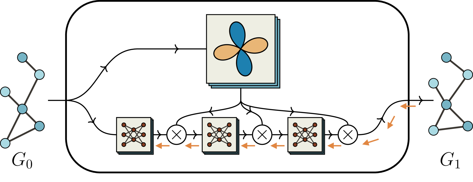
In the top half of the diagram are the equivariant basis matrices, derived from spherical harmonics. In the bottom half are trainable neural networks, which compute weights for the basis matrices. The gradient flow is shown in orange, and importantly it flows only through the neural networks and not through the basis matrices. Now compare with the simplified schematic diagram of the iterated SE(3) Transformer:

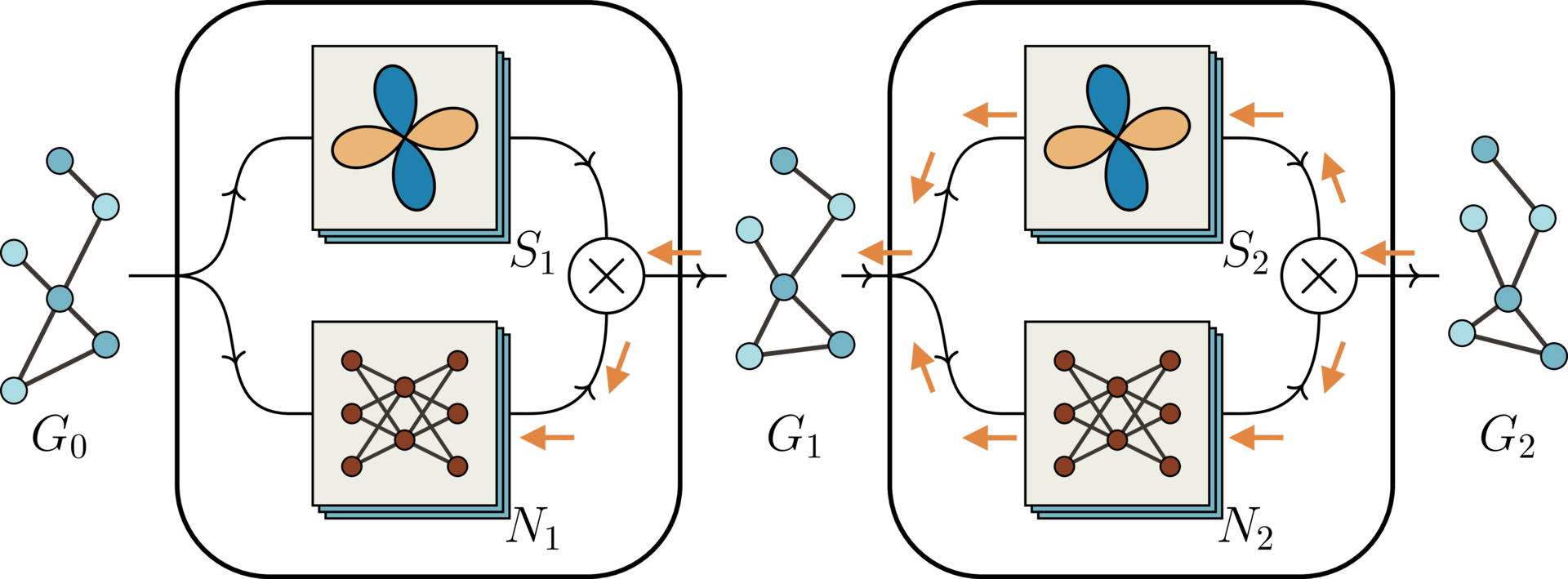
The node positions are updated after the first iteration. Since the basis matrices depend on the relative positions of the nodes, the basis matrices in the second iteration depend on the output of the first iteration. In particular, they depend on the trainable neural networks from the first iteration. This means that during training, gradients must flow back through the basis computation in the second iteration, as shown by the orange gradient flow arrows in the figure above.

Avoiding an Information Bottleneck

Naively, it seems natural for the output graph at each iteration to have the same types of features as the final output graph. However, this leads to an information bottleneck. In the intermediate layers of the SE(3)-Transformer, we can have high-dimensional fibers attached to the edges and nodes of the graph. These fibers give the network more capacity to store information about the graph – we can think of having high-dimensional fibers here as somewhat similar to having a wide intermediate layer in an MLP. In order to avoid losing this information in between iterations, the output of each intermediate iteration has the same high-dimensional fiber structure as in the intermediate layers.

Weight Sharing

It is posssible to share the trainable parameters between the iterations. This has the advantage of reducing model size and potentially mitigating overfitting. Perhaps more importantly, it allows for a flexible number of iterations with a convergence criterion. On the other hand, not sharing parameters increases the model capacity. One could argue that, in an optimsation task, this gives the model the option to actively “browse through conifguration space” instead of having to solve the same optimisation task in each iteration. In our experiments, we decided against weight sharing mainly to provide a fair comparison between iterative and single-pass SE(3)-Transformers with the same model size.

Experiment

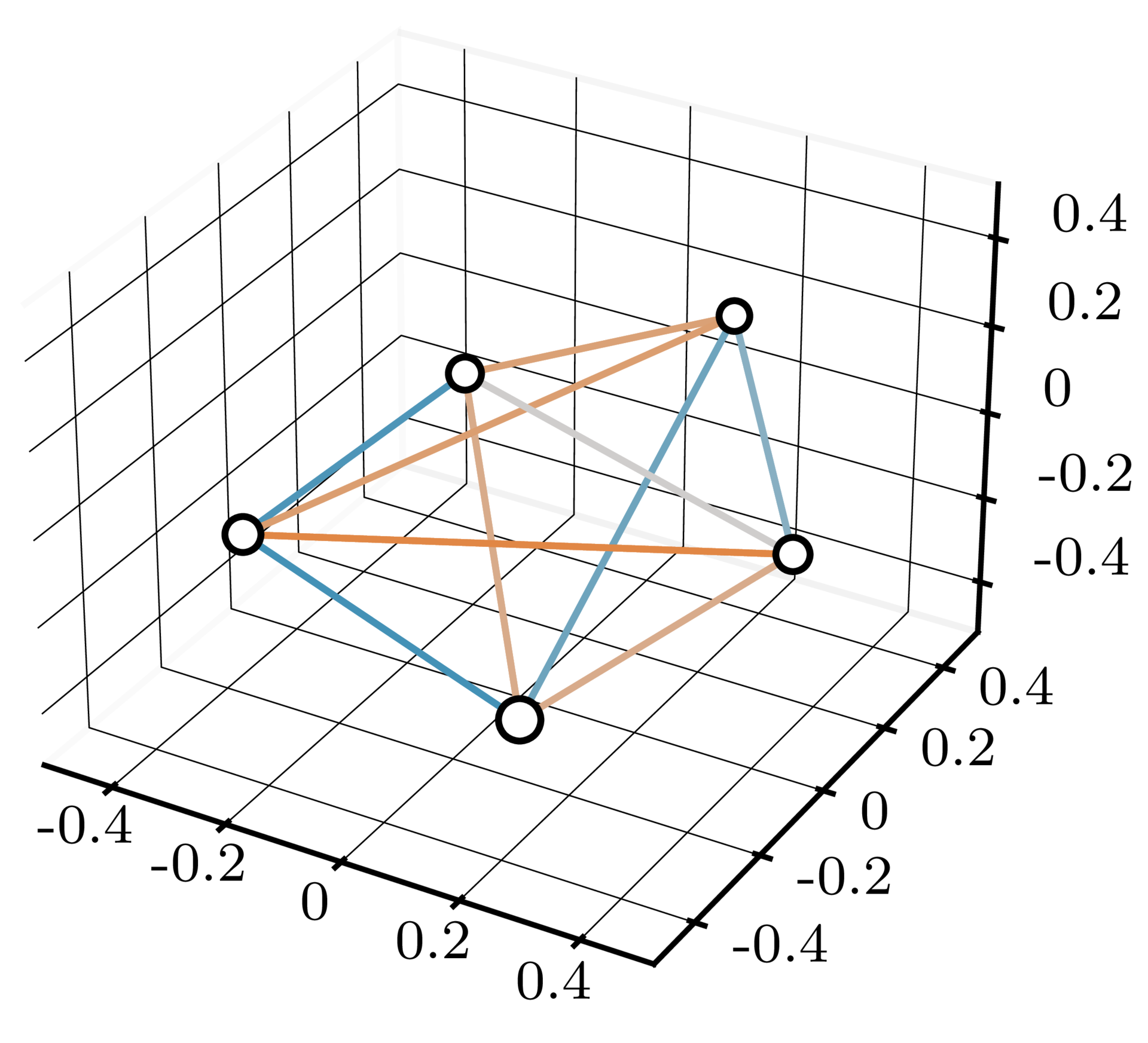
To illustrate the advantages that the iterative architecture can provide, we ran experiments on a toy problem loosely inspired by protein structure refinement. In this problem, each pair of nodes interacts according to a distance-dependent potential. Equivalently, each pair is pulled together or pushed apart by a distance-dependent force. The figure below illustrates this setup, with the force between each pair of nodes shown by the edge joining them – an attractive force is shown in orange, and a repulsive force is shown in blue.

The task is to minimise the overall potential energy of the system. This is challenging to do in one step, in part because the minimum-energy distance is different for each pair of nodes, and is unknown at input time. We trained iterative and non-iterative architectures on this task, with all architectures having the same total number of neural network layers and the same total number of parameters. We found that the iterative model outperformed the single-pass model, on average finding solutions with around $\frac{2}{3}$ the energy of the single-pass solutions. More details and findings about the experiments can be found in the report.

What We Did Not Address: Soft Sorting

When applying equivariant transformers to problems like protein structure prediction, the large number of atoms poses a challenge. Each node attending to all other nodes scales as $\mathcal{O}(N^2)$. In the original SE(3)-Transformer paper, we proposed attending only to the $K$ nearest neighbours, reducing scaling to $\mathcal{O}(K \cdot N)$. In practice, this is achieved by sorting the nodes according to distance or interaction strength. In an iterative setup, this sorting has to be redone after each position update step. In a simplified setting, the steps might be the following:

# sorting
distances, indices = torch.sort(distances, descending=False)

# take top K
indices = indices[:, :K]

# get features
features_top_K = torch.gather(features_all, dim=-1, index=indices)

Crucially, torch.gather passes gradients through features_all (hence allowing for end-to-end training) but not through indices. The fundamental issue here is that sorting is a piecewise constant function with 0 gradients almost everyone. Hence, torch.sort does not give us gradients. As a result, the network trains, but we lose part of the training signal. In other words, the network does not receive any information from the gradients about how updating the positions leads to different neighbourhood formations.

This does not mean that nothing can be done. Backpropagating through piece-wise constant functions is an established task in deep learning. The straight-through estimator, for example, could be a viable tool to apply here (Bengio et al., 2013; Yin et al., 2019). A cheap differentiable sorting operation has also been proposed by Blondel et al. (2020).

It is hard to predict whether generating additional / more complete gradient flow via soft sorting would improve the performance or harm it by polluting the information flow. Intellectually, however, this seems like a fascinating direction for future research.

Credit: Ed Wagstaff and Fabian Fuchs are funded by the EPSRC Centre for Doctoral Training in Autonomous Intelligent Machines and Systems. This blog post is based on work with Justas Dauparas and Ingmar Posner.