Explaining TrackStar from Right to Left

Training data is one of the most important ingredients in modern machine learning. It shapes what a model knows, what it fails to know, what biases it inherits, and which behaviours emerge during training. That holds for modern machine learning too, and for LLMs it maybe matters even more. But LLMs add a brutal scaling problem: their training sets contain hundreds of billions or trillions of tokens, and their predictions emerge from billions of learned parameters. At that scale, simply inspecting the data is not enough. Instead, it would be amazing to have a tool that can algorithmically connect individual model predictions back to the training examples that helped produce them. That is the problem tackled by Scalable Influence and Fact Tracing for Large Language Model Pretraining by Tyler Chang, Dheeraj Rajagopal, Tolga Bolukbasi, Lucas Dixon, and Ian Tenney, which proposes TrackStar: a gradient-based method for retrieving influential pretraining examples at LLM scale. It asks a deceptively simple question:

Which training examples most influenced this model prediction?

The paper proposes a way of asking this question at LLM-pretraining scale: compute a gradient-based representation for each training example and query, then retrieve training examples whose corrected gradients point in a similar direction.

The scale of the experiments is impressive. Chang et al. retrieve influential examples for an 8B parameter language model from a pretraining corpus of over 160B tokens, without subsampling or lexical pre-filtering. Just as importantly, the paper makes a careful conceptual distinction: examples that influence a model prediction are not always the same as examples that explicitly state the relevant fact. BM25¹ can be better at finding literal evidence; TrackStar is designed to find examples that move the model.

For a full related-work picture, see the paper itself, but it’s important to note that TrackStar is of course not inventing influence theory from scratch. The Hessian-corrected gradient product traces back to work on influence functions from Koh and Liang, while the scalable retrieval machinery builds on TracIn- and TRAK-style ideas: compare training and query gradients, approximate curvature, and use projections to make the computation feasible.

What (Not) to Expect from this Blog Post

My goal here is to build mathematical intuition for what is happening inside TrackStar. I will not give a detailed literature review or a full discussion of the paper’s empirical results. Instead, I focus on the main equation and use a small MNIST toy example I vibe-coded to make the individual pieces more tangible. The toy example is not a rigorous research project, and its findings should not be read as a comment on the paper’s results: the model, data, and scale are entirely different, and some qualitative outcomes might change, e.g., if one added the nuisance features differently. Please take it as an intuition pump, not as evidence.

The Structure of this Blog Post

This post explains the method by walking through the main equation from right to left. We start with the raw loss gradient and gradually turn it into something that can be stored, compared, and searched.

The influence score between a training example $z_m$ and a query example $z_q$ is:

\[I_\theta(z_m, z_q) = \bar{G}_\theta(z_m) \cdot \bar{G}_\theta(z_q)\]

where:

\[\bar{G}_\theta(z) = \frac{G_\theta(z)}{\|G_\theta(z)\|_2}\] \[G_\theta(z) = R^{-1/2} P_d \nabla_\theta \text{Loss}(z, \theta) / \sqrt{V}\]

In words:

Take the loss gradient for an example, correct its scale, compress it, whiten common directions, normalize it, and compare it to another example with a dot product.

The equation is dense because each term solves a different problem. The gradient tells us what the example wants the model to change. The variance correction stops a few high-magnitude parameters from dominating. The projection makes the representation small enough to store. The Hessian approximation suppresses common correlated directions. The unit normalization turns the final dot product into a cosine-like comparison of directions.

We will read this expression from right to left:

1. The raw loss gradient.
2. Division by the optimizer second moment.
3. Random projection.
4. Hessian/autocorrelation correction.
5. Unit normalization and the final dot product.

This first part covers the raw gradient and the final scoring operation, because they are the two ends of the pipeline: what signal we start with, and how we ultimately compare two examples.

1. The Raw Signal Is the Loss Gradient

The rightmost object in the TrackStar equation is:

\[\nabla_\theta \text{Loss}(z, \theta)\]

For a given example $z$, this is the gradient of the loss with respect to the model parameters $\theta$. It is a very large vector: one coordinate for each parameter of the model. Even for an 8B parameter model, this means billions of coordinates before any compression.

The idea is simple. A gradient says: if we trained on this example, which direction would it push the model? If two examples have similar gradients, then updating on one would tend to move the model in a direction that is also relevant to the other. This is the basic idea behind gradient-based influence methods.

In TrackStar, the paper computes loss gradients for both candidate training examples and query examples. For a training passage, the loss is summed over the tokens of the passage. For a query prompt and completion, only the completion tokens are used. This gives us one gradient vector for the candidate example and one gradient vector for the query.

If we had unlimited compute and storage, we could compare these full vectors directly. But full gradients are too large for LLM-scale retrieval. Even before we worry about storage, raw dot products have another problem: they are easily dominated by magnitude. Long examples, difficult examples, or examples with high-loss directions can receive large scores because their gradients are large, not because they are specifically relevant.

This is why TrackStar uses normalized vectors:

\[I_\theta(z_m, z_q) = \bar{G}_\theta(z_m) \cdot \bar{G}_\theta(z_q)\]

with:

\[\bar{G}_\theta(z) = \frac{G_\theta(z)}{\|G_\theta(z)\|_2}\]

After normalization, the dot product compares direction rather than raw length. In other words, it asks whether the training example and query would push the model in similar directions, not whether one of them simply has a very large gradient. The paper refers to the highest-scoring training examples as proponents of the query.

That gives the basic retrieval picture:

• training example → corrected gradient vector
• query example → corrected gradient vector
• dot product → influence score
• rank examples → proponents

To make this more concrete, I created a small MNIST toy example. This is not meant to reproduce LLM pretraining. It is a microscope for the individual pieces of the TrackStar equation.

The toy setup is:

• Train a small MLP on MNIST.
• Compute one loss gradient for each sampled training image.
• Compute one loss gradient for each sampled evaluation image.
• Use gradient similarity as a toy influence score.

I use two simple tests. In the first, same class vs other class, we ask whether a training image with the same digit as the eval image receives a higher influence score than a training image with a different digit. In the second, right label vs wrong label, we take the same training image twice, once with its correct label and once with an intentionally wrong label, and ask whether the correct-label gradient scores higher.

I ran this toy example in two variants. The first is clean MNIST. The second adds high-scale nuisance features that are independent of the digit label. These nuisance features are deliberately unhelpful; they are there to test whether gradient similarity can be distracted by large but irrelevant directions.

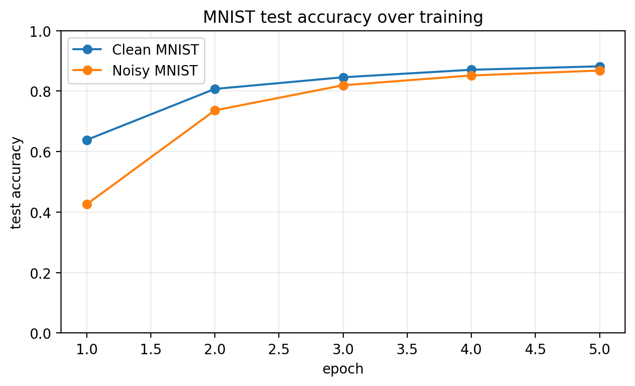
The figure above is a sanity check: before asking influence-style questions, both models have actually learned the classification task. The interesting question is not whether the classifier works, but whether the gradient geometry points to sensible examples.

The first comparison is deliberately minimal. We compare a flat, unnormalized dot product with a flat, normalized dot product. In both cases, there is no variance division, no projection, and no Hessian correction.

Setup	Scoring variant	Same-class win %	Right-vs-wrong same-label win %
Clean MNIST	Flat, unnormalized dot product	96.8	100.0
Clean MNIST	Flat, normalized dot product	100.0	100.0
Noisy MNIST	Flat, unnormalized dot product	69.2	69.6
Noisy MNIST	Flat, normalized dot product	72.8	70.8

On clean MNIST, the raw scalar product is already strong. Normalization makes it slightly cleaner, but there is not much room left to improve. The right-vs-wrong test is already at 100%, and the same-class test moves from 96.8% to 100.0%.

The noisy version is more revealing. Once high-scale irrelevant features are added, the unnormalized dot product becomes much less reliable: 69.2% on the same-class test and 69.6% on the right-vs-wrong test. Normalization improves both numbers, to 72.8% and 70.8%, but only modestly. This is exactly the situation in which the rest of the TrackStar equation becomes necessary. Directional comparison helps, but it does not by itself know which coordinates are nuisance coordinates.

2. Dividing by the Optimizer Second Moment

The next piece of the equation is:

\[\nabla_\theta \text{Loss}(z, \theta) / \sqrt{V}\]

Here, $V$ is an estimate of the second moment of the loss gradient for each model parameter. In the paper, this estimate comes from the optimizer state. The models are trained with Adafactor, and Adafactor already tracks information about the typical squared gradient magnitude of each parameter. TrackStar reuses this information to rescale the influence gradients.

The motivation is straightforward. Some parameters naturally have large gradients across many examples. If we compare gradients without correcting for this, those parameters can dominate the dot product even when they are not especially informative for the particular query. Dividing by $\sqrt{V}$ is a coordinate-wise correction: dimensions with consistently large gradient magnitudes are downweighted, while smaller but more specific dimensions get a fairer chance to matter.

This is closely related to a diagonal Hessian or Gauss-Newton correction. Rather than estimating a full curvature matrix at this stage, we first apply the simplest possible correction: one scale per parameter. The paper argues that doing this before projection is useful because it corrects individual parameters while we still have access to the full gradient.

The MNIST toy makes the reason for this step visible. Below is a diagnostic plot of gradient coordinates. The important qualitative point is that high-scale nuisance features can create large gradient components that are not actually class-specific. Note that the following plots are from the clean MNIST dataset, we don’t even need the added noise to see the effect:

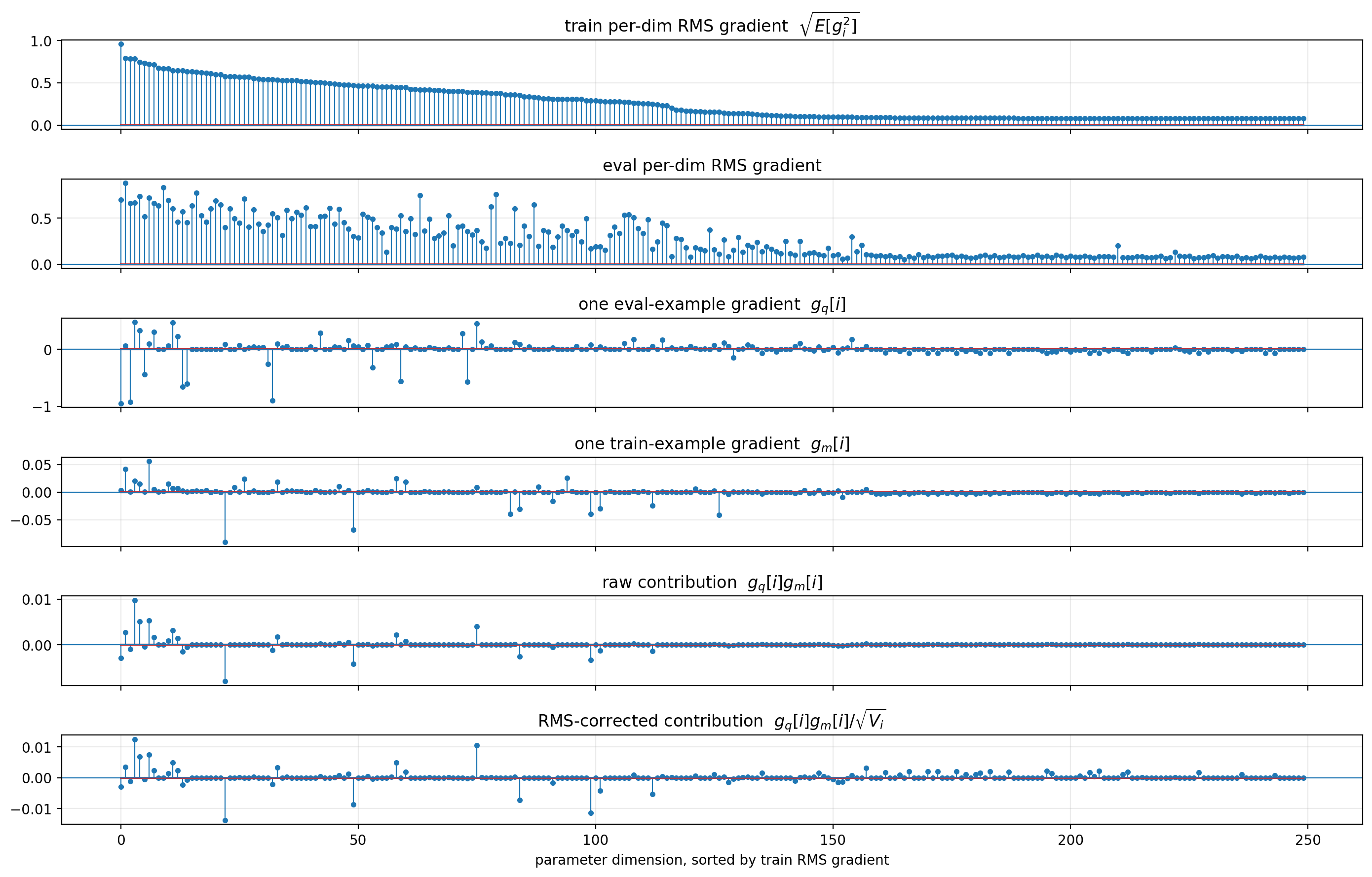
Also note that the gradients are ordered from largest to smallest training gradient, so by construction the first plot is monotonically decreasing. We can see clearly that the raw contribution (second last plot) gets no contributions to the influence score from the smaller gradients on the right. The corrected contribution (last plot), however, does.

The following table compares the flat normalized dot product before and after square-root variance division. We run it both on clean MNIST and on the nuisance version.

Setup	Scoring variant	Same-class win %	Right-vs-wrong same-label win %
Clean MNIST	Flat, no variance division	100.0	100.0
Clean MNIST	Flat, sqrt-variance division	95.4	100.0
Noisy MNIST	Flat, no variance division	72.8	70.8
Noisy MNIST	Flat, sqrt-variance division	95.4	99.7

This is a useful little stress test. On clean MNIST, variance division is apparently not needed. The gradient geometry is already aligned with the class structure, and suppressing high-variance directions can slightly hurt the same-class test. On nuisance MNIST, the picture changes. The high-scale random features distort the raw gradient geometry, and variance division brings the same-class win rate from 72.8% to 95.4%, while the right-vs-wrong win rate moves from 70.8% to 99.7%.

This is the version of the result that matches the intuition from the paper. The correction is not magic; it helps when scale is misleading. In the toy example, we deliberately create misleading scale through nuisance features. In a large language model, the corresponding problem is less artificial: transformer representations contain outlier dimensions, and optimizer state captures the fact that different parameters live at very different gradient scales.

After this step, we now have a better-scaled gradient. But for an LLM, it is still far too large to store or search over. We therefore move to the next part of the equation.

3. Random Projection Makes Retrieval Feasible

The next operation is:

\[P_d (\ldots)\]

This is the dimensionality reduction step. Even after variance correction, a full gradient for an 8B parameter model is an 8B dimensional object. TrackStar cannot store such a vector for every pretraining example, let alone compare it against thousands of queries. The paper therefore projects each corrected gradient into a much smaller space. In the main experiments, the projection dimension is:

\[d = 2^{16} = 65,536\]

A naive way to do this would be to flatten the full gradient and multiply it by one enormous random projection matrix. But for matrix-shaped neural network parameters, the paper uses a more structured alternative: two-sided random projection.

For a gradient matrix $W \in \mathbb{R}^{m \times n}$, instead of flattening $W$ and applying one large matrix, TrackStar samples two smaller random matrices and computes:

\[P_0 W P_1^T\]

If the result is $64 \times 64$, that gives $4096$ projected dimensions for that parameter block. This is mathematically a random projection of the matrix-shaped gradient, but it avoids explicitly constructing a projection matrix over all $mn$ flattened entries.

The paper applies this idea block by block. For the 8B model, gradients are grouped into eight nearby layer blocks, and attention and MLP parameters are handled separately. Each block contributes $4096$ dimensions:

\[8 \text{ layer blocks} \times 2 \text{ component types} \times 4096 \text{ dims} = 65,536 \text{ dims}\]

The main reason for doing this is computational efficiency. Two-sided projection is not primarily a claim that this representation is always more accurate than a flattened one-sided projection at the same final dimensionality. It is a way to make the projection possible at LLM scale.

The MNIST toy again gives us a small analogue. The tiny MLP has two weight matrices and two bias vectors. In the two-sided version, the weight matrices are projected into small $8 \times 8$ blocks, while the biases are projected to eight dimensions each:

• first weight matrix → 64 dims
• second weight matrix → 64 dims
• first bias vector → 8 dims
• second bias vector → 8 dims
• total → 144 dims

As a control, we also flatten the whole gradient first and apply a one-sided projection to the same final dimensionality:

• full flattened gradient → 144 dims

From here onward, I use the clean MNIST model with square-root variance division. This keeps the focus on the projection and Hessian steps rather than on the nuisance feature.

Setup	Scoring variant	Same-class win %	Right-vs-wrong same-label win %
Clean MNIST + sqrt variance	Two-sided projection	71.9	72.7
Clean MNIST + sqrt variance	Flattened one-sided projection	86.9	89.2

In this small experiment, the flattened one-sided projection preserves more of the toy influence signal. That is not a contradiction of the paper. In a small neural network, flattening the whole gradient and multiplying by a dense random matrix is perfectly feasible. For an LLM pretraining corpus, it is exactly the object we are trying not to build.

So the right interpretation is:

Projection is the compression step. Two-sided projection is the scalable matrix-aware way of doing that compression.

The quality of the compressed representation depends on the model, the task, the dimensionality, and the later corrections. In the paper, projection is only one part of the chain. The next operation, the Hessian or autocorrelation correction, changes the geometry of the projected space again. Interestingly, in our toy results, this is where the two-sided projection starts to combine more favorably with the rest of the method.

4. The Hessian Approximation

After variance correction and projection, TrackStar applies:

\[R^{-1/2}\]

This is the Hessian-like correction. The idealized influence-function expression contains an inverse Hessian term: very roughly, it asks how a small change in the training data would propagate through the learned parameters and affect the query loss. Computing the exact Hessian for an LLM is not feasible. It would be enormous, difficult to invert, and far too expensive to build over the full parameter space.

TrackStar therefore uses a projected gradient autocorrelation matrix. Let $\Phi$ be the matrix of projected per-example gradients. If we have $n$ examples and $d$ projected dimensions, then:

\[\Phi: [n, d]\] \[R = \Phi^T \Phi\] \[R: [d, d]\]

This $R$ is a Gauss-Newton-style approximation to curvature. Applying $R^{-1/2}$ whitens the projected gradients: directions that are common or highly correlated across many examples are downweighted, while more distinctive directions are relatively amplified.

The intuition is appealing. Suppose many examples share a generic feature that produces a large common gradient direction. A raw dot product may reward examples for matching this common direction, even if it is not specific to the query. The autocorrelation correction says: if this direction occurs everywhere, it should count less.

There is an important engineering detail in the paper. TrackStar does not construct one full $65536 \times 65536$ matrix. Instead, it uses a block-diagonal structure, computing smaller curvature matrices per projected block. This ignores correlations across blocks, but it makes the correction feasible. In the paper’s 8B setup, the natural block size is $4096$, corresponding to the projected dimensions for a particular layer block and component type.

In the MNIST toy, our projected gradient is only 144-dimensional, so we can look at the matrix directly:

\[\Phi: [\text{number of examples}, 144]\] \[R = \Phi^T \Phi\] \[R: [144, 144]\]

I also computed an exact projected second-derivative Hessian using Hessian-vector products. This is not what TrackStar uses at LLM scale, but it gives a useful sanity check: we can compare the paper-style autocorrelation approximation to an exact curvature object in a tiny model.

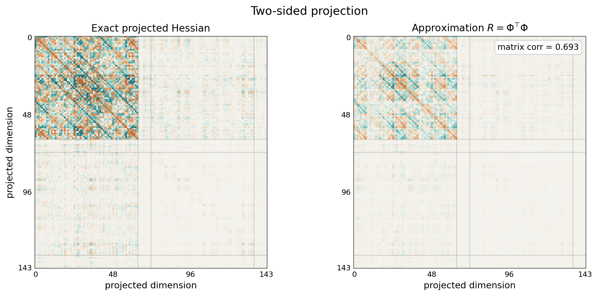
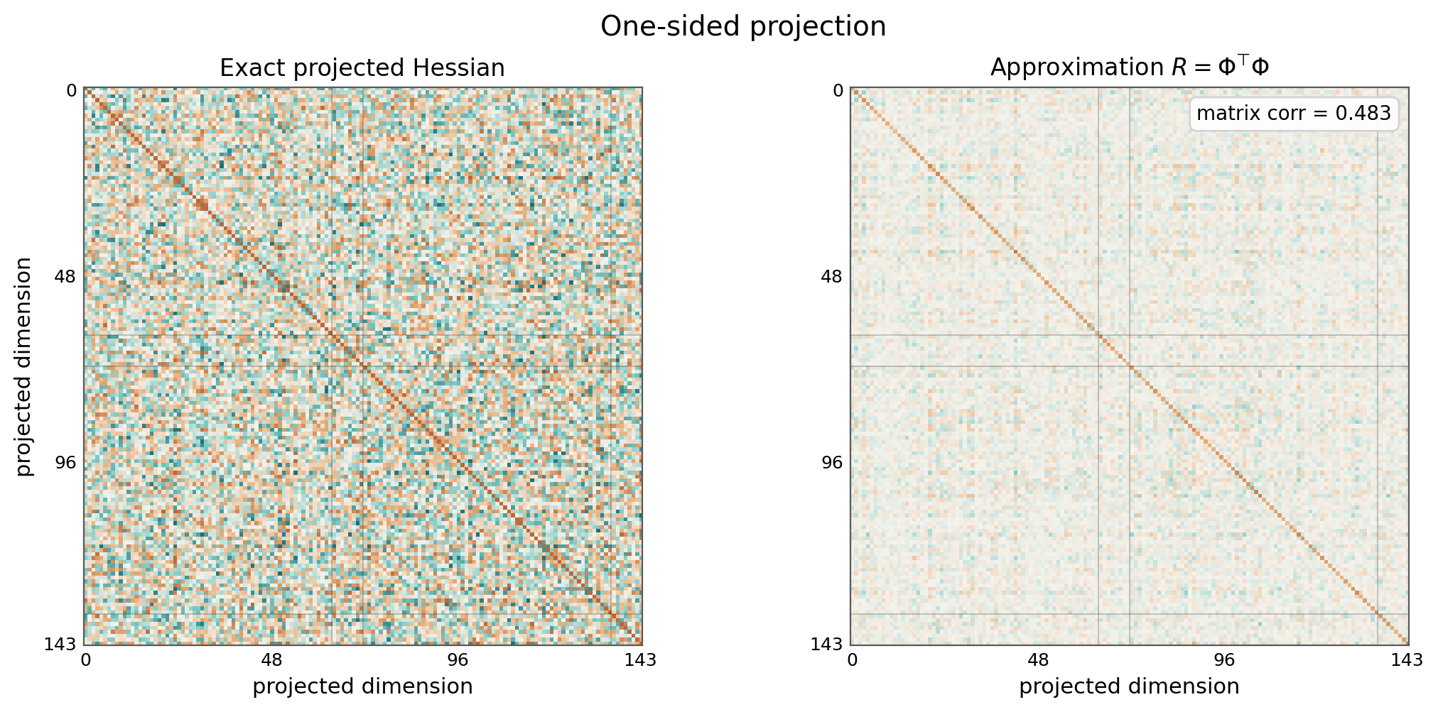
These plots are meant to be read qualitatively. The autocorrelation matrix and the exact projected Hessian are related, but they are not the same object. The approximation is attractive because it can be estimated from per-example gradients, stored in projected space, and applied symmetrically to both train and query vectors.

How does this affect the toy influence tests? Using the clean MNIST model with square-root variance division, the train-only Hessian correction gives:

Setup	Scoring variant	Same-class win %	Right-vs-wrong same-label win %
Clean MNIST + sqrt variance	Two-sided projection	71.9	72.7
Clean MNIST + sqrt variance	Two-sided projection + train Hessian	64.1	65.4
Clean MNIST + sqrt variance	Flattened one-sided projection	86.9	89.2
Clean MNIST + sqrt variance	Flattened one-sided projection + train Hessian	60.6	61.6

At first glance, this is not flattering to the Hessian step. The train-only autocorrelation correction makes both projection variants worse. This is a useful warning. Whitening is not automatically beneficial. It helps when common directions are misleading; it hurts when common directions are useful.

MNIST is exactly a setting where common directions can be useful. Many images of the same digit share broad class-level structure. If the autocorrelation correction suppresses these directions too strongly, it may remove some of the very signal we wanted to preserve. This is different from the factual prompting setup in the TrackStar paper, where many queries share task-template components that are not the specific fact being attributed.

Still, there is a small structural point worth noticing. After applying the train Hessian, the two-sided projection is now ahead of the flattened one-sided projection: 64.1% versus 60.6% on the same-class test, and 65.4% versus 61.6% on the right-vs-wrong test. Projection alone favored the flattened one-sided representation, but the Hessian correction combines better with the two-sided representation in this toy setting.

The lesson is not that the Hessian approximation always helps. Instead, my takeaway is:

The Hessian correction changes what counts as similarity. It suppresses common directions, which is useful only when those common directions are less relevant than the distinctive ones.

That distinction leads directly to the final refinement in the paper.

5. The Mixed Eval/Train Hessian

The paper does not only use a Hessian approximation computed from training examples. It also introduces a task-specific mixture:

\[R = \lambda R_\text{eval} + (1 - \lambda) R_\text{train}\]

Here $R_\text{train}$ is the autocorrelation matrix estimated from candidate training examples, while $R_\text{eval}$ is estimated from evaluation or query examples. The purpose of $R_\text{eval}$ is to identify directions that are common to the task itself.

This matters for factual prompting. If every query has a similar natural-language template, then many query gradients will share directions corresponding to the template rather than to the particular fact. A retrieval method that overweights those directions may find examples that match the task format instead of examples that are specifically influential for the target prediction.

The mixed Hessian is therefore a way to say:

Common for this task is not the same as useful for this prediction.

By mixing in $R_\text{eval}$, TrackStar downweights task-common components. The paper chooses the mixture parameter $\lambda$ so that roughly the largest task-specific components are suppressed. In their experiments, they use a stronger eval mixture for the open-set C4 retrieval setting than for the closed-set T-REx setting.

The MNIST toy only weakly exhibits this phenomenon. There is no repeated natural-language prompt template. Still, we can run the analogous experiment: compute one autocorrelation matrix from training gradients, another from evaluation gradients, mix them, and compare the result to the train-only correction.

Again using clean MNIST with square-root variance division:

Setup	Scoring variant	Same-class win %	Right-vs-wrong same-label win %
Clean MNIST + sqrt variance	Two-sided projection + train Hessian	64.1	65.4
Clean MNIST + sqrt variance	Two-sided projection + mixed eval/train Hessian	76.1	76.0
Clean MNIST + sqrt variance	Flattened one-sided projection + train Hessian	60.6	61.6
Clean MNIST + sqrt variance	Flattened one-sided projection + mixed eval/train Hessian	66.4	67.0

The mixed Hessian recovers a meaningful amount of the performance lost by the train-only Hessian. For the two-sided projection, the same-class win rate rises from 64.1% to 76.1%, and the right-vs-wrong win rate rises from 65.4% to 76.0%. For the flattened one-sided projection, the mixed correction also helps, but less strongly.

This is the cleanest version of the projection/Hessian interaction in the toy results. Before the Hessian step, flattened one-sided projection was better. After the Hessian step, and especially after mixing in eval autocorrelation, the two-sided projection is better on both tests.

The numbers should not be overinterpreted though. MNIST is not a factual language-model attribution benchmark, and it does not have the same prompt-template nuisance structure as the paper. But the qualitative point is useful: once we are no longer simply comparing projected gradients, the geometry induced by the projection can interact with the geometry induced by the Hessian correction. In this toy, the two-sided projection seems to provide a representation that works better with the whitening step.

Putting the pieces together, TrackStar’s corrected vector is:

\[G_\theta(z) = R^{-1/2} P_d \nabla_\theta \text{Loss}(z, \theta) / \sqrt{V}\]

Read right to left:

1. Compute the loss gradient.
2. Correct parameter-wise scale using the optimizer second moment.
3. Project the gradient into a manageable representation.
4. Whiten common directions using an autocorrelation-based Hessian approximation.
5. Normalize and compare with a dot product.

The resulting vectors are not literal memories of training examples. They are corrected gradient fingerprints. The paper’s contribution is to make those fingerprints scalable enough to search over a real LLM pretraining corpus.

6. Influence Is Not the Same as Evidence Retrieval

TrackStar is explicitly designed to surface training examples that causally affect a model’s prediction, whereas evidence retrieval aims to find passages that explicitly state or entail a fact. The paper evaluates both objectives: factual retrieval (MRR, recall@10) measures whether retrievals contain entailing passages, while the tail-patch experiment measures how much a retrieved example increases the model’s probability of the target answer.

Empirically, classical lexical retrievers (BM25) and dense embedding methods (Gecko) score higher on factual retrieval: they more reliably return entailing passages and thus obtain higher MRR/recall. TrackStar, by contrast, retrieves examples that produce larger tail-patch effects—i.e., examples that actually move the model’s probabilities more, even when those examples do not lexically entail the fact.

This mismatch is the paper’s central empirical finding: examples that explicitly state a fact are not always the most causally influential. Influential examples can be entailing, but they can also be partial matches, passages that reinforce priors or relation-type signals, or other contexts that change model behavior. The authors further show that factual retrieval and influence tend to become more aligned as models and training tokens scale, though the gap does not vanish.

Practical takeaway: use lexical or embedding retrievers (e.g., BM25, Gecko) when the goal is to find explicit evidence; use TrackStar when the goal is to identify which training examples actually drove the model’s behavior. The two approaches are complementary.

Closing Takeaway

TrackStar starts with an object that is too large and too noisy to use directly: the full loss gradient of an example with respect to a large language model. It then turns that object into a searchable representation:

\[G_\theta(z) = R^{-1/2} P_d \nabla_\theta \text{Loss}(z, \theta) / \sqrt{V}\]

Read from right to left, each piece has a role.

The loss gradient says what the example would change in the model. The optimizer second-moment correction reduces misleading parameter-scale effects. The random projection makes the representation small enough to store and search. The Hessian/autocorrelation correction suppresses common correlated directions. Finally, unit normalization and a dot product turn the corrected gradients into a retrieval score.

The MNIST toy is useful because it separates these ingredients. Raw gradients already carry influence signal. Normalization helps when magnitude starts to matter too much. Variance division becomes important when high-scale nuisance features distort the geometry. Projection is mainly about feasibility. The Hessian step is subtle: it helps when common directions are nuisance directions, but can hurt when common directions are useful class signal. Mixing eval and train autocorrelations is a way to downweight task-common structure more deliberately.

The full paper applies this chain at a much larger scale. It retrieves proponents for an 8B parameter language model from a pretraining corpus of over 160B tokens. The result is not merely a bigger retriever. It is a method for asking a sharper question:

Which training examples would actually move the model toward this prediction?

That question is close to evidence retrieval, but not the same. Sometimes the influential example states the fact. Sometimes it supports a prior, a relation, a name, or a partial association. This is precisely why influence methods are useful: they expose the difference between what looks like evidence to us and what functions as evidence inside the model.

---